Timing Synchronization in OFDM Systems

Orthogonal Frequency Division Multiplexing (OFDM) has been the vehicle driving most high rate wireless communication systems in the world today. Some of the notable examples are our WiFi, 4G and 5G technologies. See the interesting LoRa PHY for modulation techniques based on frequency shift – chirp spread spectrum that utilize many of the concepts from OFDM for algorithm design.

As a background, we have also discussed before the impact of a timing error on an OFDM signal. It was observed that an integer timing offset does have affect the performance as long as it within certain boundaries. A fractional timing offset introduces a phase rotation that becomes part of the complex channel gain. Therefore, the purpose of a timing recovery scheme in OFDM is to ensure that the FFT window starts from within the region of correct samples.

Today we explore how timing synchronization can be achieved in an OFDM system. For this purpose, the correlation operation is mostly employed in an explicit manner for time domain estimation of synchronization parameters.

The discussion is mostly based on the synchronization techniques in Ref. [1], commonly known as Schmidl and Cox synchronization for OFDM.

Training Correlation

---

First, consider the correlation of a pseudo-random sequence of $+1$s and $-1$s with itself (i.e., autocorrelation) for several time shifts (there are many specialized sequences available for this purpose such as Gold codes and Kasami codes but since optimization is not our purpose, we consider a random stream of $+1$s and $-1$s here). The summation in the correlation of such a long stream of opposite signs will mostly cancel out and the resultant value will be large only when they exactly coincide. From the article on AWGN, we know that the autocorrelation of white noise is a unit impulse. When we draw the autocorrelation of a pseudo-random sequence in the figure below for a range of negative and positive time shifts, we can see that such a sequence approximately behave like noise due to the resulting impulse generation. The important result is that the autocorrelation of this sequence has a sharp peak when completely aligned, much higher than any other time shift.

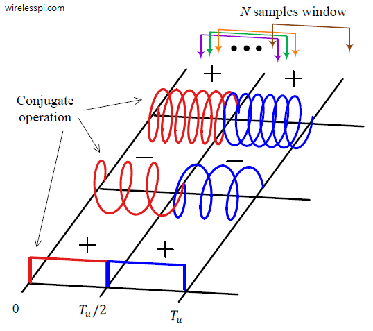
Second, two copies of such a pseudo-random sequence is prepended before the data symbols without any iFFT at the Tx, i.e., the training sequence is in time domain. The Rx is sampling the signal in the expectation of the OFDM frame. Here, the initial samples are composed of just noise, followed by the above training sequence and then the OFDM symbols as illustrated in the figure below. We choose an initial sample and compute the correlation as follows.

If a sample in $z[n]$ is multiplied with the conjugate of another sample spaced $N/2$ apart, and $N/2$ such multiplications are carried out and summed together, then this will yield a large value only when this starting sample coincides with the start of the training sequence. An example of such a correlation is shown in the figure below for a length $N=4$ training sequence composed of $\{+,-,-,+\}$.

• In the top figure above which illustrates a wrong location for the correlation start, assume that the two noise samples have a $-$ and $+$ sign, respectively. Then, the correlation result here (normalized by $1/N$) becomes
  \begin{equation*}
  \frac{1}{4}\sum \Big\{(-\cdot +), ~(+\cdot -),~(-\cdot -), ~(+\cdot +)\Big\} = 0
  \end{equation*}

  One could argue that the noise samples could have opposite signs and hence generate a large value. But remember that we are considering an example for a very small $N=4$. For a large value of $N$, it is improbable that so many noise samples have exactly the same signs in succession as the training sequence. Furthermore, the example is taken near the training sequence where the last two values in the window are already the same due to the presence of a CP. This partial similarity gives rise to a gradually increasing slope of the correlation result, instead of a sharp peak.

• Next, we shift this correlation window by $1$ sample to the right and compute the $N/2$-spaced correlation among the samples falling within this window. And continue repeating this process.
• When this correlation window reaches the actual frame start, i.e., the initial sample of the training sequence, the following result is produced.
  \begin{equation*}
  \frac{1}{4}\sum \Big\{(+\cdot +), ~(-\cdot -),~(-\cdot -), ~(+\cdot +)\Big\} = 1
  \end{equation*}

  which corresponds to the exact alignment of the length $N/2$ training sequence. Connect this result with the impulse in the figure before the last one that illustrates $\delta[n]$ as its autocorrelation.

The Coarse Timing Metric

---

To form such a signal, we construct a single OFDM symbol that consists of the length $N/2$ iFFT of a pseudo-random sequence, i.e., the training sequence is in frequency domain now and consists of complex samples. Then, we repeat it twice in time domain which makes the second half of this OFDM symbol the same as the first half. This forms our training sequence prepended at the start of an OFDM frame consisting of two identical halves with length $N/2$ each.

Note that such a training sequence can also be generated by assigning the length $N/2$ sequence to even subcarriers and zeros to odd subcarriers. This is equivalent to upsampling by $2$ the length $N/2$ sequence in frequency domain. Therefore, its length $N$ FFT is composed of two copies in the time domain, just like upsampling by $P$ in time domain consists of $P$ spectral replicas in frequency domain.

After the addition of a CP, the convolution of the channel will affect both halves of the training sequence in a similar manner. The samples received are denoted as $z[n]$ and let us compute a correlation in this sequence in the following manner. Utilizing the definition of correlation, we define the index $\epsilon_0$ as the sample where the correlation starts and a metric $P(\epsilon_0)$ based on this index as
\begin{equation}\label{eqOFDMpd}
P(\epsilon_0) = \sum_{i=0}^{N/2-1} z\left[\left(\epsilon_0+\frac{N}{2}\right)+ i\right]z^*\left[\epsilon_0+i\right]
\end{equation}

This correlation involves a window of $N$ samples starting at $\epsilon_0$ that slides to the right while searching for the training symbol. The conjugate operation is necessary to rotate the length $T_u/2$ subcarriers in the first half in an opposite direction to cancel them out and add the signs of the pseudo-random sequence in a coherent manner. This is drawn in the figure below where a length $N$ correlation window is also visible for the ideal correlation start.

There are two factors that can cause a wrong timing offset if only $P(\epsilon_0)$ is used for this purpose.

Phase/frequency rotation

---

Recalling that OFDM is a passband and hence complex modulation scheme and the subcarriers are composed of both $I$ and $Q$ components, $P(\epsilon_0)$ in Eq \eqref{eqOFDMpd} above consists of complex samples. How should we compare this metric for different values of $\epsilon_0$, through the $I$ part, $Q$ part or the magnitude? If there is a phase rotation between the two identical halves of the training symbol, the in-phase part will not produce a correct amount of correlation. For a worst case phase offset of $\pi/2$ between them, a zero appears at the $I$ output while all the correlation magnitude appears in the $Q$ output.

Similar is the case when a frequency offset is present in the Rx signal that spins the modulation symbols and makes the two identical halves non-identical. Observe that if this was not the case, then the best method to acquire the timing is to correlate the incoming signal (in which the training is embedded) with a locally stored copy of the training at the Rx which is free of noise and other distortions. The presence of a frequency offset ruins the correlation of two otherwise identical sequences. One simple remedy for this problem is to focus on the magnitude squared of the metric $P(\epsilon_0)$.

Signal energy

---

Since the channel is not AWGN, the Rx signal energy can vary throughout the duration of the transmission. Consider a case where the energy is high in the first half and low in the second half. Consequently, the correct peak will exhibit a low value and hence can be easily missed even for the correct $\epsilon_0$. The solution here is to normalize the metric $P(\epsilon_0)$ with the energy of the samples within the correlation window. However, each sequence in the correlation consists of $N/2$ samples, so only $N/2$ samples need to be taken into account. While energy in any of the two halves can be measured, the second half is usually chosen as a precaution against an unexpectedly long channel.
\begin{equation*}
E(\epsilon_0) = \sum_{i=0}^{N/2-1} \left|z\left[\left(\epsilon_0+\frac{N}{2}\right)+ i\right]\right|^2
\end{equation*}

Taking into account the above two factors, a new timing synchronization metric can be defined as
\begin{equation}\label{eqOFDMmd}
M(\epsilon_0) = \frac{|P(\epsilon_0)|^2}{\left[E(\epsilon_0)\right]^2}
\end{equation}

And the optimal timing instant $\hat \epsilon_0$ (recall that timing synchronization in OFDM corresponds to locating the correct sample, i.e., an integer offset) is given as
\begin{equation}\label{eqOFDMoptimalTiming}
\hat \epsilon_0 = \max _{\epsilon_0} M(\epsilon_0)
\end{equation}

Here, the denominator $E(\epsilon_0)$ can be considered as a virtual AGC to provide a suitable signal gain for accurate timing metric detection. A block diagram of such an implementation is illustrated in the figure below. We will later come back to this scheme in another article to find out how it helps in coarse CFO correction.

Recursive Implementation

---

The main attraction of such a strategy is the correct result even in the presence of the CFO due to the magnitude squared operations involved. Furthermore, from a hardware point of view, such a timing metric can be implemented in a recursive manner thus simplifying its implementation. For this purpose, write $P(\epsilon_0+1)$ from Eq \eqref{eqOFDMpd} as
\begin{equation*}
P(\epsilon_0+1) = \sum_{i=0}^{N/2-1} z\left[\left(\overline{\epsilon_0+1}+\frac{N}{2}\right)+ i\right]z^*\left[\overline{\epsilon_0+1}+i\right]
\end{equation*}

This is the same correlation window as computed for $\epsilon_0$ but shifted by $1$ sample to the right. Therefore, the leftmost sample (corresponding to $i=0$) can be excluded from $P(\epsilon_0)$ and an additional sample from the right (corresponding to $i=N/2$) can be added to $P(\epsilon_0)$ to get $P(\epsilon_0+1)$.
\begin{align*}
P(\epsilon_0+1) &= \underbrace{\sum_{i=0}^{N/2-1} z\left[\left(\epsilon_0+\frac{N}{2}\right)+ i\right]z^*\left[\epsilon_0+i\right]}_{P(\epsilon_0)} – z\left[\epsilon_0+\frac{N}{2}\right]z^*\left[\epsilon_0 \right] + \\
&\hspace{1.7in}z\left[\epsilon_0+N\right]z^*\left[\epsilon_0+\frac{N}{2}\right]
\end{align*}

Similarly, the denominator $E(\epsilon_0)$ can be recursively computed as
\begin{equation}\label{eqOFDMrecursiveTiming}
E(\epsilon_0+1) = E(\epsilon_0) – \left|z\left[\epsilon_0+\frac{N}{2}\right]\right|^2 + \left|z\left[\epsilon_0+N\right]\right|^2
\end{equation}

For these reasons, such a correlation window is implemented in most of the OFDM receivers for timing synchronization purpose.

Improvements on the Timing Scheme

---

We have seen above an implementation of a coarse timing estimation scheme through autocorrelation, i.e., correlation between the samples of the same sequence. When such a timing synchronization scheme is implemented for an OFDM frame in which there is a training sequence prepended at the start, we get the timing metric $M(\epsilon_0)$ of Eq \eqref{eqOFDMmd} drawn in the figure below for $N=512$ subcarriers, a $25\%$ CP, a random training sequence and an AWGN channel. Notice that as the correlation window slides past the OFDM signal, the timing metric gradually rises near the training, reaches a plateau when the window hits the CP, remains constant for the duration of the CP (25%) and then slides down gradually after the training begins.

Since this is an AWGN channel, there is no ISI within this plateau to distort the signal and the first sample can be taken anywhere within this region. This was shown earlier here as a region of no concern. In a frequency selective channel, the length of this plateau is actually given as
\begin{equation*}
\text{Plateau length} = \text{CP length} – \text{channel length}
\end{equation*}

In an AWGN channel, the plateau is as long as the CP.

The next question is how to utilize the timing metric $M(\epsilon_0)$ for synchronization purpose. The most straightforward way is to raise a flag of preamble detection whenever $M(\epsilon_0)$ rises past a certain threshold. However, the metric possesses a flat timing plateau instead of exhibiting a sharp peak. Moreover, due to this flat plateau, the variance of the timing synchronization estimate is quite high. For reliable operations and exact analysis, we like to have a repeatable experience with as less a variance as possible.

Many variations on this timing synchronization scheme have been proposed, some of which we discuss next.

Peak detection through $90\%$ points

---

While a naïve solution is to find the maximum point $\varepsilon_{0,\text{max}}$ of $M(\epsilon_0)$, this is not a reliable solution as well since it will move around in each realization due to the random noise. A better solution in Ref. [1] is to detect the peak by finding this maximum point, then locate the points to the left and right of this maximum value that are $90\%$ of this maximum value, and average the time points corresponding to these two $90\%$ values.

Smoothing with a moving average filter

---

With the knowledge that the plateau has a maximum length equal to the CP in an AWGN channel, the flatness of this region can be turned into a linearly rising curve by convolving it with a moving average filter having a length equal that of the CP. The rationale is that a flat signal resembles a rectangular signal and convolution of a rectangle with another rectangle in the moving average filter is a triangle that exhibits a relatively pronounced peak.

Such a modified metric is plotted in the above figure where the single point of the sequence start can be isolated. Note that the convolution result is not a triangle because the plateau is not a rectangular signal in isolation. In any case, with the peak of the timing metric $M(\epsilon_0)$ in hand, many peak finding strategies — similar to the symbol centric and zero crossing techniques — can also be applied if a long frame of OFDM symbols is available and convergence time is not much of a concern. This happens for example in continuous transmission systems.

Repetitions with the same or different signs

---

An interesting alternative technique to improve the timing metric $M(\epsilon_0)$ in Eq \eqref{eqOFDMmd} is as follows. Consider the training sequence with $2$ identical halves as a special case of a training sequence with $L$ repetitions as well as different signs. For example, denote the length $N/2$ training sequence by $A$. Then, until now, we have worked on a sequence $A$ repeated twice and with $++$ signs, as illustrated in the top figure below. By $++$ sign, we do not mean the signs of the individual training symbols before the iFFT but that the whole length $N/2$ sequence $A$ after the iFFT is multiplied with a $+1$ to generate $\{+A,+A\}$.

Now consider the bottom figure above where a training sequence with $L=4$ identical parts is drawn. While the underlying training before the length $N/4$ iFFT is the same, each iFFT output quarter is multiplied with a different pattern, $\{-A,+A,-A,-A\}$ in this case, and concatenated together. The advantage of such an approach is that even after the insertion of the CP, there is no plateau left due to the presence of only one unique time shift for which the whole correlation window exactly matches. The timing metric $M(\epsilon_0)$ is still given by the ratio of $P(\epsilon_0)$ and $E(\epsilon_0)$ but both of these metrics are modified to implement the summation of products between the samples of the repetitive parts. This is shown in the figure below where the logic of sign inversion responsible for the steep rolloff of the timing metric is also evident. We will see in another article how such a strategy is useful for CFO estimation as well.

It must be kept in mind that during the computation of $P(\epsilon_0)$, the actual repetitive pattern (e.g., $\{-A,+A,-A,-A\}$) must be multiplied with the corresponding training part for canceling its sign. Figure below compares the timing metric $M(\epsilon_0)$ for $L=4$ repetitions with the pattern $\{-A,+A,-A,-A\}$ and original $L=2$ repetitions employing the pattern $\{+A,+A\}$. It is evident that the plateau has disappeared and a steep rolloff of the timing metric helps in locating the exact timing sample for synchronization purpose. The concept demonstrated here for $4$ repetitions can be easily generalized to $L$ repetitive parts.

Let us now return towards the preamble of IEEE 802.11a standard.

Example

---

In 802.11a standard for WiFi, the preamble consists of a Short Training Field (STF) with $10$ repetitions and a Long Training Field (LTF) with $2$ repetitions. This is drawn below where $S$ represents the short training field. Other than coarse timing synchronization, the STF is also utilized for several different purposes (e.g., signal detect, Automatic Gain Control (AGC), diversity selection and coarse frequency synchronization). The LTF consists of two identical halves used for fine frequency synchronization as well as channel estimation while a GI2 represents a guard interval of twice the normal length.

The STF in 802.11a is generated by taking an iFFT of the sequence below. Notice that only a few subcarriers from $k=-26$ to $k=+26$ are employed for this purpose which are multiples of $4$, the effect of which we shortly see. From $k$ $=$ $-26$ to $+26$,
\begin{align*}
a_{\text{STF}}[k] = \sqrt{\frac{13}{6}}\bigg\{ &0, 0, \underbrace{+V}_{-24}, 0, 0, 0, \underbrace{-V}_{-20}, 0, 0, 0, \underbrace{+V}_{-16},0, 0, 0, \underbrace{-V}_{-12}, 0, 0, 0,\\ & \underbrace{-V}_{-8}, 0, 0, 0, \underbrace{+V}_{-4}, 0, 0, 0, \underbrace{0}_{0}, 0,
0, 0, \underbrace{-V}_{+4}, 0, 0, 0, \underbrace{-V}_{+8}, 0, \\ &0, 0, \underbrace{+V}_{+12}, 0, 0, 0, \underbrace{+V}_{+16}, 0, 0, 0, \underbrace{+V}_{+20}, 0, 0, 0, \underbrace{+V}_{+24}, 0, 0\bigg\}
\end{align*}
where $V$ is a complex number given by
\begin{align*}
V_I\: &= 1 \\
V_Q &= 1
\end{align*}

The scaling factor $\sqrt{13/6}$ comes from normalizing the average power of the OFDM symbol which employs $12$ out of $52$ available subcarriers. Combined with $\sqrt{1/2}$ that is used to make $V$ above a unit energy number,
\begin{equation*}
\sqrt{\frac{1}{2}\cdot\frac{52}{12}} = \sqrt{\frac{13}{6}}
\end{equation*}

What is the implication of only the subcarriers in STF being multiples of $4$ utilized for modulation purpose? This can be seen as a case of upsampling a signal consisting of $13$ values by $4$. From multirate signal processing, we know that upsampling by inserting $L$ zeros in one domain causes a repetition by $L$ in the other domain. In frequency domain, this repetition was visible in the form of the $L$ spectra becoming a part of the upsampled signal spectrum. Here, the zero insertion is in frequency domain and hence $L=4$ repetitions appear in time domain. The time duration of the iFFT output is the FFT size $N$ multiplied with the sample time $T_S=1/20\times 10^6$ $=$ $50$ ns. Thus, the time period of one repetition consisting of $64/4=16$ samples is given by
\begin{equation*}
\frac{NT_S}{4} = \frac{64 \times 50\times 10^{-9}}{4} = 0.8 \mu \text{s}
\end{equation*}

and the total duration of the STF field is $10\times 0.8=8\mu$s. As another example, the LTF is generated through the iFFT of the following symbols.
\begin{align*}
a_{\text{LTF}}[k] = \Big\{&1, 1, -1, -1, 1, 1, -1, 1, -1, 1, 1, 1, 1, 1, 1, -1,
-1, 1,\\ &1, -1, 1, -1, 1, 1, 1, 1, 0, 1, -1, -1, 1, 1, -1,
1, -1, 1, \\&-1, -1, -1,-1, -1, 1, 1, -1, -1, 1, -1, 1, -1, 1, 1, 1, 1\Big\}
\end{align*}

Observe that all $52$ subcarriers are utilized. There are numerous other metrics and even more variations on those metrics that have been discovered in the enormous research literature on OFDM systems. Nevertheless, the fundamental concepts remain similar to what has been discussed above.

An interested reader can study the intriguing training sequences defined in various standards implementing the OFDM systems such as WiFi (802.11a/g/n/ac), WiMax (802.16), LTE (4G), NR (4.5G) and 5G systems.

• Once a coarse timing estimate $\hat \epsilon_0$ is located, it is also customary to advance it by a predetermined number of samples as a safety margin against channel dispersion. Recall from the discussion on the effect of STO that taking the FFT between the ideal sampling instant and the point where the channel ends has no effect on the demodulator performance because any residual phase becomes part of the channel phase $\measuredangle H[k]$ for each $k$. This safety margin introduces a cushion in synchronization design where an advance of a few samples can be afforded but not a delay of even $1$ sample.
• As a final remark, we have established the necessity of some kind of periodicity in the Rx signal to mark the timing synchronization instant. For OFDM systems consisting of long packets or continuous transmissions such as DAB or DVB, the timing synchronization can be accomplished through using the cyclic prefix which is essentially a short repetition in an OFDM symbol. Nevertheless, the underlying concepts related to building useful metrics and defining thresholds remain unchanged. For example, the timing metric using a CP can be written as
  \[
  P_{CP}(\epsilon_0) = \sum_{i=-N_{CP}}^{-1} z\left[\left(\epsilon_0+N\right)+ i\right]z^*\left[\epsilon_0+i\right]
  \]

  where the repetition happens at a time difference of $N$ samples and gives rise to a high correlation. The other two metrics, namely $R(\epsilon_0)$ and $M(\epsilon_0)$, can also be defined in a similar manner. Keep in mind that for one length $N$ OFDM symbol, the sample indices including the CP are defined as follows.
  \begin{equation*}
  -N_{CP}, \cdots,-1,0,1,2,\cdots,N-1
  \end{equation*}

Fine Timing Synchronization

---

The coarse timing offset above was computed through using the autocorrelation, i.e., correlation between the samples of the same sequence. Advantages of this approach are its computational complexity due to recursive structure in Eq \eqref{eqOFDMrecursiveTiming} and that it is immune to any impairment caused by the CFO. Nonetheless, the disadvantage of such an approach is that both sets of samples are noisy and hence the performance remains suboptimal.

One remedy to this problem is that we already have a ‘clean’ copy of the training sequence stored at the Rx. Why not correlate the noisy Rx signal with the stored clean sequence? Recall that the noisy version of the training is affected by the CFO and hence even its correlation with the clean sequence will be rotating instead of generating a single sharp peak.

To solve this issue, a coarse frequency offset is also computed after the coarse timing estimation and compensated for which we describe in a later article. Once the noisy Rx sequence is mostly free of the coarse CFO, we denote it by $\tilde z[n]$ and a fine timing estimate is computed by cross-correlating it with the clean training sequence $s[n]$ stored at the Rx. The new metric $\tilde{M}(\epsilon_0)$ is given by
\begin{equation*}
\tilde{M}(\epsilon_0) = \sum_{n=0}^{N-1} \tilde z\left[n+\epsilon_0\right]s^*\left[n\right]
\end{equation*}

Such a strategy is also known as matched filtering because the correlation is implemented with the known training sequence $s[n]$. In practice, such a cross-correlation produces highly accurate results. To reduce the acquisition time, this operation can be carried out partially with a portion of $s[n]$ as well. For IEEE 802.11a example, after the coarse timing computation from the Short Training Field (STF), a partial correlation with $32$ or $64$ samples of the Long Training Field (LTF) can be carried out instead of the complete length $128$ sequence for a fine timing estimate.

On the other hand, in the continuous or frame-based OFDM systems, fine timing can be accomplished through averaging over a number of OFDM symbols. This is because the acquisition time requirements are relevantly much more relax as compared to packet based systems and a simple tradeoff between extending the averaging interval for an increased accuracy is feasible.

References

[1] T. Schmidl and D. Cox, "Robust frequency and timing synchronization for OFDM," IEEE Trans. Commun., vol. 45, Dec. 1997