Timing synchronization is one of the most fascinating topics in the field of digital communications. The impact of symbol timing offset has been discussed in the context of single-carrier systems before.
The intuition behind how an OFDM system works is also presented in a previous article.
However, the problem of timing synchronization is quite different in OFDM systems as compared to single-carrier systems due to the nature of the waveform. Let us explore how a timing error impacts the demodulated waveform in such a scenario.
To avoid using many indices, we skip the OFDM symbol index $m$ in the following expressions to focus on each OFDM symbol. Moreover, upconversion and downconversion through a carrier at frequency $F_C$ is also bypassed and complex baseband representations are employed. Finally, no additive white Gaussian noise is present to study the effects of each impairment in isolation.
Constructing an OFDM Waveform
For a bit stream $b[k]$ mapped to a non-binary modulation scheme $X[k]$ (having I and Q components), an OFDM signal $s[n]$ can be constructed through an inverse Discrete Fourier Transform (iDFT) operation as
\[
v[n] = \frac{1}{N} \sum \limits _{k=-N/2} ^{N/2-1} a[k] e^{j2\pi \frac{k}{N}n}
\]
which is a representation in terms of complex signals. See the tutorial on OFDM for an intuitive understanding of why this expression generates the desired waveform.
In terms of real signals, this baseband OFDM signal at the Tx can be written as
$$
\begin{equation}
\begin{aligned}
v_I[n]\: &= \frac{1}{N}\sum \limits _{k=-N/2} ^{N/2-1}\left[ a_I[k] \cos 2\pi\frac{k}{N}n – a_Q[k] \sin 2\pi\frac{k}{N}n\right] \\
v_Q[n] &= \frac{1}{N} \sum \limits _{k=-N/2} ^{N/2-1} \left[a_Q[k] \cos 2\pi\frac{ k}{N}n + a_I[k] \sin 2\pi\frac{k}{N}n\right]
\end{aligned}
\end{equation}\label{eqOFDMiDFT2}
$$
Keep in mind that the data symbols $a[k]$ arise from a linear modulation scheme in exactly the same manner as in single-carrier systems but are assumed to be in frequency domain here due to the iFFT operation involved.
After the digital to analog conversion, what is the form of the continuous-time signal? Clearly, the expression for subcarriers in continuous domain is $2\pi F_k t$ where each subcarrier frequency $F_k$ in Hz is given by
\[
\begin{aligned}
F_k = \frac{k}{NT_S} = k\Delta_F \qquad \text{for each }k = -N/2,\cdots,N/2-1
\end{aligned}
\]
where we have used the fact that an OFDM symbol duration is given by $N$ samples at a sample rate of $1/T_S$ that defines the period (and hence frequency $\Delta_F$) of the lowest frequency sinusoid. The above relation comes from the definition of discrete frequency and reinforces the concept that the subcarrier frequencies $F_k$ should be integer multiples of subcarrier spacing $\Delta_F$. Now from $F_kt$ in continuous time domain, the OFDM signal in continuous-time becomes
\[
\begin{aligned}
v_I(t)\: &= \frac{1}{N}\sum \limits _{k=-N/2} ^{N/2-1}\left[ a_I[k] \cos 2\pi F_kt – a_Q[k] \sin 2\pi F_kt\right] \\
v_Q(t) &= \frac{1}{N} \sum \limits _{k=-N/2} ^{N/2-1} \left[a_Q[k] \cos 2\pi F_kt + a_I[k] \sin 2\pi F_kt\right]
\end{aligned}
\]
The spectrum of such an OFDM signal is drawn in the figure below. Notice the rectangular structure within the spectrum and sinc like sidelobes at the edges. To constrain the spectrum, a time domain Raised Cosine (RC) pulse shape can also be used.

With zero noise, the same signal is received at the Rx convoluted by the channel and the baseband version is denoted by $x(t)$.
Role of Carrier Frequency and Timing Offsets
Before we sample $x(t)$ to go to the discrete domain, we need to know how a Carrier Frequency Offset (CFO) $F_ \Delta$ and a Symbol Timing Offset (STO) $\epsilon _\Delta$ affects the Rx signal. For this purpose, let us focus on the expression $F_kt$. After the synchronization errors, this becomes
\[
2\pi F_k t \quad \xrightarrow \quad 2\pi (F_k +F_ \Delta)(t+\epsilon _\Delta)
\]
After sampling at a rate of $F_S=1/T_S$, we can write
\begin{equation*}
\begin{aligned}
2\pi(F_k +F_ \Delta)(t+\epsilon _\Delta)\big|_{t=nT_S} \quad &= 2\pi\left(F_k + F_ \Delta\right)\left(nT_S+\epsilon _\Delta\right) \\
&= 2\pi\left(F_k + F_ \Delta\right)\left(n+\frac{\epsilon _\Delta}{T_S}\right)T_S \\
&= 2\pi\frac{F_k + F_ \Delta}{F_S} \left(n+\frac{\epsilon _\Delta}{T_S}\right) \\
&= 2\pi\left(\frac{F_k}{F_S} + \frac{F_ \Delta}{N\Delta_F} \right)\left(n+\frac{\epsilon _\Delta}{T_S}\right) \\
&= \frac{2\pi}{N}\left(k + \frac{F_ \Delta}{\Delta_F} \right)\left(n+\frac{\epsilon _\Delta}{T_S}\right)
\end{aligned}
\end{equation*}
where we have used $F_k=k\Delta_F$ and
\begin{equation*}
\frac{1}{\Delta_F} = NT_S = \frac{N}{F_S} \quad \Rightarrow \quad F_S = N\cdot \Delta_F
\end{equation*}
Also, $F_ \Delta/\Delta_F$ (where $F_ \Delta$ here is the CFO and $\Delta_F$ is the subcarrier spacing) and $\epsilon _\Delta/T_S$ are normalized CFO and STO, respectively, as encountered before in the context of single-carrier systems. We denote them by
\begin{equation*}
\nu_0 = \frac{F_ \Delta}{\Delta_F} \qquad \epsilon_0 = \frac{\epsilon _\Delta}{T_S}
\end{equation*}
With these settings in place, the above expression can be modified as
2\pi(F_k +F_ \Delta)(t+\epsilon _\Delta)\big|_{t=nT_S} ~~ = \frac{2\pi}{N}\left(k + \nu_0 \right)\left(n+ \epsilon_0\right)
\end{equation}
Now we can use the above relation to get the sampled baseband version of the Rx signal $x[n]$ which after lowpass filtering produces the signal $z[n]$. Skipping the mathematical details of this process, all we need to do is include the product of a channel coefficient $H[k]$ with data symbol $a[k]$ for each subcarrier $k$ into Eq \eqref{eqOFDMiDFT2}. Defining $Z[k] = a[k]H[k]$ as a product between the data modulation and channel gain,
\[
\begin{aligned}
z_I[n]\: &= \frac{1}{N}\sum \limits _{k=-N/2} ^{N/2-1}\Big[ Z_I[k] \cos \frac{2\pi}{N}(k+\nu_0)(n+\epsilon_0) – \\
&\hspace{1in}Z_Q[k] \sin \frac{2\pi}{N}(k+\nu_0)(n+\epsilon_0)\Big]
\end{aligned}
\]
\[
\begin{aligned}
z_Q[n] &= \frac{1}{N} \sum \limits _{k=-N/2} ^{N/2-1} \Big[Z_Q[k] \cos \frac{2\pi}{N}(k+\nu_0)(n+\epsilon_0) + \\
&\hspace{1in}Z_I[k] \sin \frac{2\pi}{N}(k+\nu_0)(n+\epsilon_0)\Big]
\end{aligned}
\]
For a zero CFO and STO, the above equation is just an iDFT of $Z[k]$. If you are familiar with complex notations in OFDM, you can recognize this equation as
\begin{equation*}
z[n] = \frac{1}{N}\sum_{k=-N/2}^{N/2-1} a[k]H[k] \exp\left(j\frac{2\pi}{N}(k+\nu_0)(n+\epsilon_0)\right)
\end{equation*}
Hence after the DFT at the Rx, we get our $Z[k]$ back which are the modulation symbols $a[k]$ scaled by the channel coefficients $H[k]$.
We conclude that the timing synchronization problem in OFDM systems is slightly different than single-carrier systems. There, a symbol timing offset is the fractional interval between $0$ to symbol time $T_M$ due to the necessity of just $1$ sample/symbol for symbol detection. Here, while the sample/symbol is still $1$, these symbols are grouped into $N$ samples of an OFDM symbol. Consequently, there is an integer part of the Symbol Timing offset (STO) and a fractional part.
Integer Symbol Timing Offset
The integer part of the STO problem corresponds to locating the right sample. What exactly is the right sample? A major portion of the processing at the Rx is composed of taking the $N$-point DFT (actually, FFT) of the incoming signal. For this purpose, the Rx must know the starting sample of the sequence which will form the input to this FFT routine. This samples coincides with the end of the cyclic prefix and constitutes of the useful portion of the OFDM symbol $NT_S$. As a result, all $N$ samples participate in estimating the location of the right sample. This availability of $N$ samples/OFDM symbol implies that the (OFDM) symbol timing synchronization problem is quite similar to the frame synchronization part in the single-carrier systems. This is shown in the figure below where the boundaries of the OFDM symbols in an OFDM frame are drawn for clarification purpose. The task of the timing synchronization unit is to locate these boundaries.

Fractional Symbol Timing Offset
As far as the fractional part of the STO is concerned, it is a bit surprising but we do not really need to estimate it. Recall from the DFT of a time shifted signal that a delay in time domain induces a frequency dependent phase shift in frequency domain.
\[
\text{Time shift} \quad s[(n\pm n_0) \:\text{mod}\: N] \quad \rightarrow\quad \pm 2\pi \frac{k}{N} n_0 \quad \text{Phase shift}
\]
Consequently, after the DFT, the fractional timing offset appears as a phase rotation at each individual subcarrier $k$ and hence becomes part of the phase of the channel gain $H[k]$. Since we were not slicing the spectrum in separate subcarriers in single-carrier systems, we could not apply this result there for rate $1/T_M$ sampling. But the timing phase offset does become part of the channel phase for a fractionally-spaced equalizer, enabling it to compensate for this timing phase. A timing recovery loop, however, is still required to track the waveform periodicity in the form of clock frequency.
Exploring the Limits
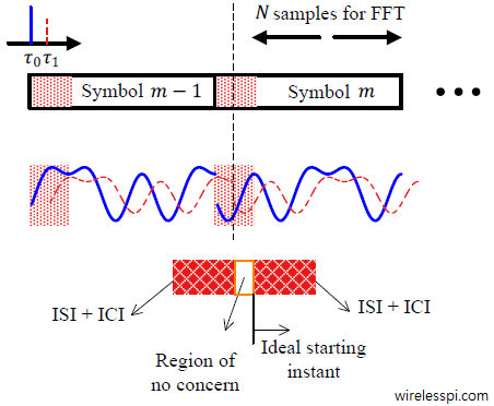
The question now is the following: how far away the timing offset can be from the ideal sampling instant such that no ISI or ICI is contributed in the DFT input. For this purpose, refer to the figure below that shows two OFDM symbols in succession.

- The ideal sampling instant is the sample where the Cyclic Prefix (CP) ends. However, even if our first sample is behind this location, there is no harm done as long as it lies after the contamination from the previous symbol (i.e., beyond the channel length). Carefully look at the waveform portion of the above figure. In this region of no concern, only the multipath copies of the same subcarrier are being summed up for each subcarrier and this can only induce a change in phase. This change in phase merges into the channel phase $\measuredangle H[k]$ which is compensated by the equalizer later.
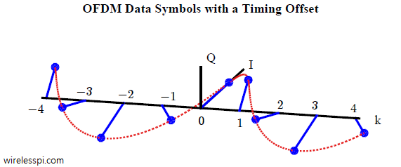
- If the STO $\epsilon_0$ is within this region, and a DFT is computed at the Rx, we know from our knowledge of time frequency duality that the effect of a timing error on an OFDM symbol should cause a spinning of the symbols defined in frequency domain, just like a carrier frequency offset in a single-carrier system rotated the constellation of our symbols defined in time domain.
Therefore, after the DFT, the Rx symbols will be rotating in circles with an inverse period $\epsilon_0$ (whether it is an integer or a fraction), as long as $\epsilon_0$ is within the region of no concern. This is drawn in the figure below.
- To confirm our intuition, we manipulate the argument of the subcarriers at the Rx FFT input in Eq \eqref{eqOFDMfreqTimeOffsets}, reproduced below, as follows.
\begin{align*}
2\pi(F_k +F_ \Delta)(t+\epsilon _\Delta)\big|_{t=nT_S} ~~ &= \frac{2\pi}{N}\left(k + \nu_0 \right)\left(n+ \epsilon_0\right) \\
&= \frac{2\pi}{N} \left\{ \underbrace{kn}_{\text{Term 1}} + \underbrace{\nu_0 n}_{\text{Term 2}} + \underbrace{k \epsilon_0}_{\text{Term 3}} + \underbrace{\nu_0 \epsilon_0}_{\text{Term 4}} \right\}
\end{align*}- From the DFT definition, we know that the FFT at the Rx consists of subcarriers with the arguments $-kn$ which simply cancels out Term 1 above.
- Term 2 appears as a normalized CFO at the FFT output because it is a function of time $n$.
- Term 4 is neither a function of $n$ nor a function of $k$. Hence, it appears as a constant phase that gets merged into the channel phase $\measuredangle H[k]$.
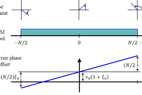
- This leaves Term 3 as a function of STO and clearly it is being multiplied with the subcarrier index $k$. As a result, the data symbols at each subcarrier $k$ get rotated by the product of this index $k$ varying from $-N/2$ to $N/2-1$ with the STO $\epsilon_0$ and this is what causes the constellation rotation. In other words, these data symbols are multiplied with a complex sinusoid $2\pi(k/N)\epsilon_0$ with inverse period $\epsilon_0$ and we see this complex sinusoid rotating in frequency domain in the figure below, which is exactly the same as drawn in figure before in the form of a scatter plot.
- Referring back to the above figure depicting the cyclic prefix, when the starting sample of the OFDM symbol is before the region of no concern, the subcarriers from the previous OFDM symbol interfere with the current OFDM symbol inducing both ISI and ICI.
- Finally, when the input window is after the ideal sampling instant, then a similar ISI and ICI come from the next OFDM symbol.


Next Steps
Having established the necessity to have synchronization in place, we have also explored the most prevalent estimation technique, commonly known as Schmidl and Cox synchronization. Keep in mind that in the single-carrier systems, our Master Algorithm, the correlation, was mostly employed in an implicit manner in the sense that the fundamental expression was derived from the correlation and then various approximations were found to estimate the desired parameter. In the case of OFDM, the correlation is overwhelmingly utilized in an explicit manner for time domain estimation of synchronization parameters.