In the article on beamforming, we discussed the interaction of the electromagnetic waves with the antenna array without any description of what the beam shape looks like. As we explore below now, the beam shape is given by the Fourier Transform of individual antenna intensities but the reason behind this is not always explained in most of the textbooks and tutorials on this topic. Where exactly does the Fourier Transform, a conversion tool from time $t$ to frequency $\omega=2\pi F$ domain, come into the picture? And how does the frequency $\omega$ for time domain correspond to phase shift $u$ of the array elements?
Coming back to our analogy between time domain and space domain sampling, let us find out the cumulative radiation pattern of a linear arrangement for a group of antennas. This is commonly known as the array factor of a linear array and it can be derived through the techniques borrowed from time to frequency transformation. The starting point is a rectangular signal in time domain shown below.

Main Lobe in Frequency Domain
The tool we use for going into frequency domain is the Discrete-Time Fourier Transform (DTFT). It defines the spectral representation of a signal $x[n]$ as
\[
\begin{aligned}
X_I(e^{j \omega})\: &= \sum \limits _{n}\bigg[ x_I[n] \cos \omega n + x_Q[n] \sin \omega n\bigg] \\
X_Q(e^{j \omega}) &= \sum \limits _{n}\bigg[ x_Q[n] \cos \omega n – x_I[n] \sin \omega n\bigg]
\end{aligned}
\]
where $ \omega$ is the discrete frequency variable. The complex version of this definition is shown below.
In terms of complex signals, the DTFT is defined as
\begin{equation}\label{equation-dtft-complex}
X(e^{j \omega}) = \sum _n x[n] e^{-j \omega n}
\end{equation}
For a rectangular pulse as shown above, $x[n]$ is an all-ones sequence.
\begin{equation}\label{equation-dtft-rect}
X(e^{j \omega}) = \sum _n e^{-j \omega n}
\end{equation}
The frequency response or spectrum of a rectangular pulse is derived here as
\begin{equation}\label{equation-rect-sinc}
\big|X(e^{j\omega})\big| = \frac{\sin N\frac{\omega}{2}}{\sin \frac{\omega}{2}}
\end{equation}
The above spectrum is known as an aliased sinc signal that includes the aliases arising from finite sample rate (we have a violation of sampling theorem here because spectrum of a rectangular signal is a sinc signal that has infinite bandwidth). As $N$ becomes large (i.e., sample rate goes to infinity), we can apply the approximation $\sin A \approx A$ in the denominator and the spectrum approaches that of an actual sinc signal. This is drawn in the figure below where a main lobe appears at index $0$ while the sidelobes decay as we move away from zero on either side. Keep in mind that as more samples are collected, the main lobe of the sinc signal becomes more concentrated around index 0.

Spectral Filtering
With the discrete-time samples available, DSP algorithms can be applied to modify the output spectrum in frequency domain as desired. This is known as spectral filtering. Interestingly, even a simple sinc filter shown in the figure above has a lowpass response! It passes the frequencies around zero with little distortion and blocks the frequencies further away. We can say that it acts as a spectral filter.
The main lobe of the sinc signal does not have be at zero frequency. Recall the modulation property of Fourier Transform according to which multiplication of individual samples with a complex sinusoid in time domain shifts the signal in frequency domain.
Let us reproduce the frequency domain version of the time shift property here.
\begin{equation}\label{equation-frequency-shift-property}
x[n]\cdot e^{j\omega_o n} \quad \stackrel{\mathrm{FT}} {\longleftrightarrow}\quad X((e^{j (\omega-\omega_0}))
\end{equation}
We see that multiplying the signal $x(t)$ with the samples of a complex sinusoid shifts the spectrum at $\omega_0$.
This is plotted in the figure below where the main lobe of the sinc has been shifted to $\omega=\pi/2$ as a result of such multiplication. Now the frequencies around that value can pass unhindered but rest of the frequencies, both above and below, are attenuated. We have a bandpass response. For a practical implementation with low sidelobe levels in the spectrum, there are several techniques, such as windowing (e.g., Hamming, Blackman-Harris, Kaiser-Bessel), that can be applied to the time domain signal.

Main Lobe in Spatial Domain
This is an interesting idea due to the analogy between samples in time forming a sinc signal and samples in space forming a directional beam. If each antenna exhibits an ideal omnidirectional pattern, then their equal intensities can be represented as a series of constants. Now when each antenna successively delays its waveform, the resultant field formed at any angle $\theta$ in space comes from their superposition in that direction! The mathematical expressions are as below.
Recall the article on beamforming that describes the antenna phase shift for each successive element.
\begin{equation}\label{equation-u-def}
u = \omega \tau = 2\pi \frac{d\sin\theta}{\lambda}
\end{equation}
where the variable $u$ is the spatial counterpart of the frequency variable $\omega$ in time sampling.
Recall that a complex sinusoid $e^{j\omega t}$ delayed by $\tau$ is given by $r_1(t)=e^{j\omega (t-\tau)}$. This can be generalized to form $r_n(t)$ and when signals from $N$ array elements are added together with their respective delays, we have
\begin{align*}
\text{Superposition of Waves} = \sum_n r_n(t) = \sum _n e^{j\omega (t-\tau_n)} =& e^{j\omega t} \sum _n e^{-j\omega \tau_n} \\=& e^{j\omega t} \sum _n e^{-j u n}
\end{align*}
where the last step follows from the definition of $u$ in Eq (\ref{equation-u-def}). The first factor above is the input sinusoid and the second is known as the array factor (AF) defined as
\begin{equation}\label{equation-array-factor-1}
\text{AF} = \sum _n e^{-j u n}
\end{equation}
Compare the above expression with Eq (\ref{equation-dtft-rect}). They are very similar! This is the reason why directional response of an antenna array is given by the Fourier Transform of the array amplitude distribution. In words, we have seen that time delays for narrowband signals can be represented as products with complex scalars and hence their superposition at any point in space can be written as a sum of those complex scalars!
For a uniform intensity distribution of the isotropic case, we can simply write the array factor with the help of Eq (\ref{equation-rect-sinc}) as
\begin{equation}\label{equation-array-factor-2}
\text{AF} = \frac{\sin N\frac{u}{2}}{\sin \frac{u}{2}}
\end{equation}
This is also an aliased sinc signal but in space domain! Let us now see some figures related to this concept.
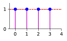
- The equal weight given by each antenna in spatial direction is shown as a constant signal in the figure below, the same as an array emitting a continuous wave with uniform amplitude distribution.
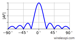
- The array factor with respect to phase shift $u$ is drawn in the figure below which approaches a sinc signal for large $N$.
- The overall radiation pattern is the product between the individual antenna pattern and the array factor as drawn in the figure below.
\[
\text{Overall Pattern} ~=~ \text{Element Pattern} \times \text{Array Factor}
\]The array factor is an interesting characteristic of the system because it arises from a particular configuration of participating elements and acts beyond their individual radiation patterns (this also helped me understand why a group, team, organization or a nation is not a simple sum of their parts, e.g., why organizations with efficient employees might not be productive). Keep in mind that for non-planar arrays (such as a base station with a circular or ring array) in general, the element pattern cannot be factored out of the cumulative expression.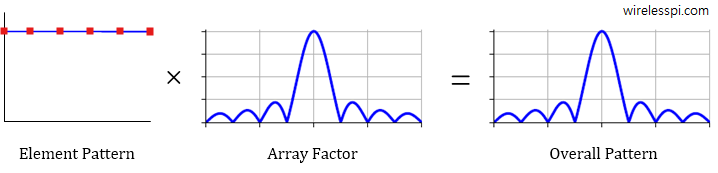
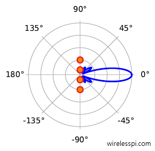
- When this sinc signal is bent into a polar pattern just like you wear a belt around your waist, a beam is formed where the main lobe points in a given direction: $u=0$ in this case. This is drawn in the figure below.
- Continuing from the frequency shift analogy in time domain samples that was shown earlier, individual samples in space domain (i.e. antenna inputs or outputs) can be multiplied with a complex sinusoid to shift the beam direction in spatial domain as illustrated in the figure below.
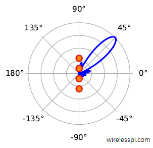


Spatial Filtering
Analogous to spectral filtering we saw before, the beams in space can be shifted to produce a desired spatial response where the larger lobe produces a higher gain. Signals arriving from one or more directions can be blocked or passed by careful design of these complex multipliers. This is known as spatial filtering. Furthermore, just like the windowing functions in time domain, the beam can be modified with reduced sidelobe levels through analogous weighting functions.
Role of Number of Elements $N$
Let us now observe the behavior of the antenna array for the number of elements $N$ with antenna spacing $d$. For this purpose, the coming figures plot the array factor $|AF|$ introduced in Eq (\ref{equation-array-factor-2}) at a frequency of 60 GHz by varying $N$ and $d$. We observe the following.
- Drawn in the figure below is the array factor for $N=4$ antennas at a spacing of $d=\lambda/2$. A single wide main lobe of a sinc function is visible in the look range of $\theta=-90^\circ$ to $+90^\circ$. Let us determine the zero crossing locations with respect to beam direction $\theta$. For this purpose, notice that the numerator and denominator in Eq (\ref{equation-array-factor-2}) are both zero at $u=0$.
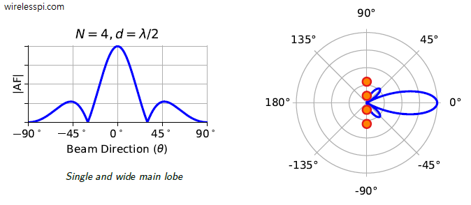
Therefore, the array factor magnitude crosses zero again when the numerator $Nu/2$ becomes $\pi$. This yields
\[
u=\frac{2\pi}{N}
\]
Plugging in the value of $u$ from Eq (\ref{equation-u-def}),
\begin{equation}\label{equation-zero-crossing}
2\pi \frac{d\sin\theta}{\lambda} = \frac{2\pi}{N}
\end{equation}
For $d=\lambda/2$, this turns out to be
\[
\sin\theta = \frac{2}{N}
\]
For $N=4$, our first zero crossing appears where $\sin\theta=1/2$. Consequently, it can be located in the figure above at $\theta=\sin^{-1}(1/2)=30^\circ$. The main lobe width is twice this value.The right side of the above figure shows the same function bent into a polar pattern. We say that the array has a main beam at $0^\circ$ or it transmits and receives maximum amount of energy at $0^\circ$.
- When the number of elements is increased from $N=4$ to $N=8$, the sinc main lobe becomes narrow. Plugging $N=8$ with $d=\lambda/2$ in Eq (\ref{equation-zero-crossing}), we get $\theta=14.5^\circ$ as seen in the figure below.
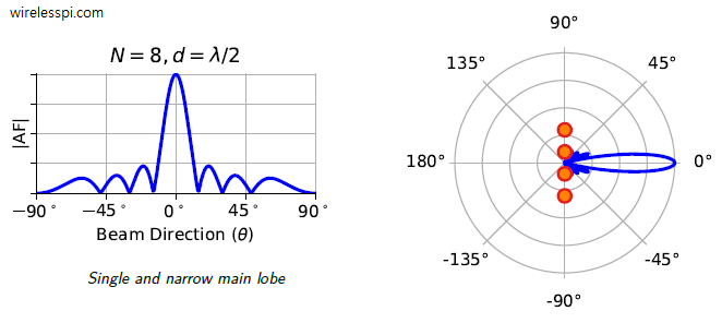
The effect of increase in $N$ is visible on the right side polar plot with a narrower beam. In systems where users are separated in spatial dimension, these narrow beams result in less interference, both within the same signal (ISI) and from the remaining users.


Role of Antenna Spacing $d$
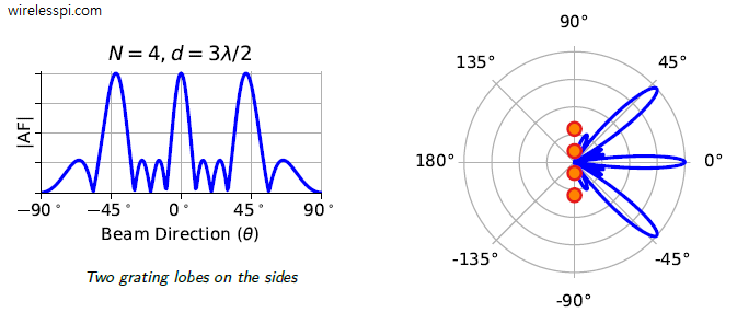
Increasing the number of elements $N$ is not the only way to achieve narrow beams. Let us fix the number of elements $N=4$ and modify the antenna spacing $d$ to $3\lambda/2$. The resulting array factor is drawn in the figure below where one can observe a narrower main beam as compared to $d=\lambda/2$. Why two new lobes have arisen will be discussed shortly.

The first zero crossing can be derived as before from Eq (\ref{equation-zero-crossing}). Plugging $N=4$ and $d=3\lambda/2$, we have
\[
\sin \theta = \frac{2}{3N} = \frac{1}{6}
\]
Here, $\theta$ turns out to be $9.6^\circ$. Shown on the right side is the polar plot with this narrow beam even though the number of elements is still $N=4$. We realize the following.
It was observed that the beamwidth (here, null-to-null spacing of the main lobe) depends on both the number of elements $N$ and antenna spacing $d$. Looking back, we can see that the real parameter of interest here is the array length $L$ that is a product of these two variables. The array length is defined as
\[
L=(N-1)d
\]
which you can easily verify by looking at a uniform linear array. On a side note, I personally like to view the array length as $L=Nd$ due to the analogy from time domain sampling. Recall from here that a discrete-time pulse with $N$ samples at a spacing of $T_S$ is said to have a length of $NT_S$ because going into discrete spectrum virtually constructs periodic copies starting at time $NT_S$ (which has the same signal value as time $0$). This is known as input periodicity of the Discrete Fourier Transform (DFT). Furthermore, many derivations in analysis of antenna arrays are simplified by taking the length as $Nd$ instead of $(N-1)d$.
Returning to the additional two lobes in the figures above, these are called grating lobes that are similar to aliases in frequency domain arising from violating the spatial sampling theorem as $d=3\lambda/2$. Recall the sampling theorem in time domain, $T_S\le 1/2B$ where $B$ is the signal bandwidth. We can thus write an analogous expression as
\[
d \le \frac{\lambda}{2}
\]
The exact relationship for this spacing for a reference look direction $\theta_0$ of the array is derived here as
\[
d \le \frac{\lambda}{1+\sin \theta_0}
\]