Once upon a time, an antenna was viewed as a simple device to transmit and receive an electromagnetic wave, much like a battery the sole purpose of which is to provide electrical power. A set of antennas, however, can be viewed from a new angle as follows.
Sampling in Time Domain
An Analog-to-Digital Converter (ADC) is a device that samples an analog signal in time domain to create a corresponding sequence of numbers. Similarly, a Digital-to-Analog Converter (DAC) gets a sequence of numbers as an input to generate a reconstructed analog signal. As an example, a rectangular pulse shape is shown in the figure below which is sampled at regular intervals separated by $T_S$ seconds. The length of the pulse is equal to one symbol interval in continuous time domain.
\begin{equation*}
T_M = N T_S
\end{equation*}

Observe that an interval of length $N T_S$ seconds is not the same as the interval covered by $N$ samples with a separation of $T_S$ seconds between them. In discrete-time, the pulse length contains $N$ samples with a total length of $(N-1)T_S$ seconds but the missing sample in the end is the same as the first sample of the next pulse if they were transmitted in a continuous stream. Therefore, the pulse length is given by $N\cdot T_S$ as above. This point seems trivial but it is quite important in understanding the length of an antenna array.
The sampling interval $T_S$ is chosen according to the bandwidth $B$ of the arriving signal. Sampling theorem in DSP tells us that the sampling rate $F_S=1/T_S$ required to capture all the information in an analog signal should be greater than twice the bandwidth $B$, or $1/T_S \ge 2B$. In other words, the spacing between two samples $T_S$ should be less than half the inverse bandwidth.
\begin{equation}\label{equation-sampling-theorem}
T_S \le \frac{1}{2B}
\end{equation}
For a sinusoidal wave as an example, we require at least two samples within each cycle. The question now is how to choose the right sample spacing $T_S$.
- If $T_S$ is chosen as much smaller than in the above expression (a high sample rate), then we have many more samples to process than required. This adds to the system cost through extra storage and signal processing as well as reduced efficiency.
- On the other hand, a value for $T_S$ greater than $1/2B$ implies a violation of sampling theorem. This gives rise to aliasing in frequency domain which are spectral replicas of the original waveform appearing within the band. A set of aliases arising as a result of aliasing is shown in the figure below.

Sampling in Space Domain
In a manner analogous to sampling by the ADC and reconstruction by the DAC in time domain, the signals arriving at an antenna array can be visualized as being sampled in space domain. Similar to the discrete-time sampling, the bottom part of the figure below depicts an antenna array sampling the signal at a regular spacing of $d$ meters.

Here, the spacing $d$ between the elements is chosen according to the wavelength $\lambda$ of the target signal. Similar to sampling theorem in time domain, we have the following relation
\[
d \le \frac{\lambda}{2}
\]
This is called critically spaced antenna spacing and corresponds to the time domain condition $1/2B$. In practice, there is another condition for the spacing between antenna elements.
\begin{equation}\label{equation-antenna-spacing}
d \le \frac{\lambda}{1+\sin \theta_0}
\end{equation}
where $\theta_0$ is the direction of the array pattern peak. Why is there a difference between $\lambda/2$ and the above expression? As we see in the derivation below, this is because the directional response of the array as a result of spatial sampling is analogous to frequency response in time sampling but the correspondence is between the sine of angle, $\sin(\theta)$, instead of $\theta$ alone and the frequency variable $\omega=2\pi F$ during the transformation. Feel free to skip the derivation in the box.
- Start with a general reference angle $\theta_0$ to gauge the response with respect to that direction. The phase shift at the first antenna (where the wave reaches after a delay of $\tau$) is given by
\[
u = \omega \tau =2\pi F \frac{d\sin \theta_0}{c} = 2\pi \frac{d}{\lambda}\sin \theta_0
\]because the wave travels an extra distance of $d\sin \theta$ with respect to reference antenna 0, as explained in the discussion on beamforming. We have also utilized $c= F\lambda$ where $c$ is the speed of an electromagnetic wave.
- Directing to a desired angle $\theta$ implies adjusting $u$ as
\[
u = 2\pi \frac{d}{\lambda}\Big(\sin \theta – \sin \theta_0\Big)
\] - Assuming $\theta_0\ge 0$, the maximum for $|u|$ occurs at $\theta=-\pi/2$ given by
\[
|u|_{\text{max}} = 2\pi \frac{d}{\lambda}\Big(1+\sin \theta_0\Big)
\] - The Fourier Transform of a sequence of samples with equal magnitudes (i.e., a rectangular pulse) is given by a sinc signal.
\[
AF = \frac{\sin N\frac{u}{2}}{\sin \frac{u}{2}}
\]This tells us that the denominator is zero only at $u=0$ where the numerator is also zero. This forms the maximum gain that can be found in the limit. However, the position of grating lobe lies where this maximum is reached again, i.e., both the numerator and the denominator are again zero. This happens for $u=2\pi$.
- There are no grating lobes as long as $|u|_{\text{max}}$ is less than this value.
\[
2\pi \frac{d}{\lambda}\Big(1+\sin \theta_0\Big) \le 2\pi
\]This leads us to the final expression.
\begin{equation}\label{equation-antenna-spacing-der}
d \le \frac{\lambda}{1+\sin\theta_0}
\end{equation}
Figure below illustrates this concept for a main lobe that points at $\theta_0=30^\circ$ for $N=32$ antennas at the frequency $F=60$ GHz. Can you guess the element spacing $d$ just by looking at the figure?

Sine the grating lobe has just started to appear at the left edge, the relation in Eq (\ref{equation-antenna-spacing-der}) is at the boundary, i.e., it satisfies the equality. With $\theta_0=30^\circ$, we have
\[
d = \frac{\lambda}{1+\sin(30^\circ)} = 0.67\lambda
\]
We conclude the following.
- If the antenna spacing $d$ is lesser than the above value, it is like collecting more samples in space than necessary. Such a small spacing is expensive from a hardware viewpoint, increases mutual coupling and reduces spatial diversity between channels.
- If the spacing is larger than the above value, then there are less number of elements for the same array length that reduces manufacturing costs and the associated feeding circuitry. Nonetheless, these advantages come at the cost of grating lobes, a phenomenon similar to spectral aliases for time domain sampling. Suffice it to say here that the normal operation of an array is to pick up signals from desired directions and attenuate the rest. Instead, grating lobes pick up signals from some undesired directions as well without attenuation.
In the light of the above, the goal is to design antenna arrays with the widest possible spacing until the effect of grating lobes starts to appear. The relation in Eq (\ref{equation-antenna-spacing}) is derived for the peak of the grating lobe, not the middle between the main and grating lobes. Therefore, many multiple antenna systems are designed as a series of identical elements separated by a distance of $0.5\lambda$ to $0.7\lambda$.
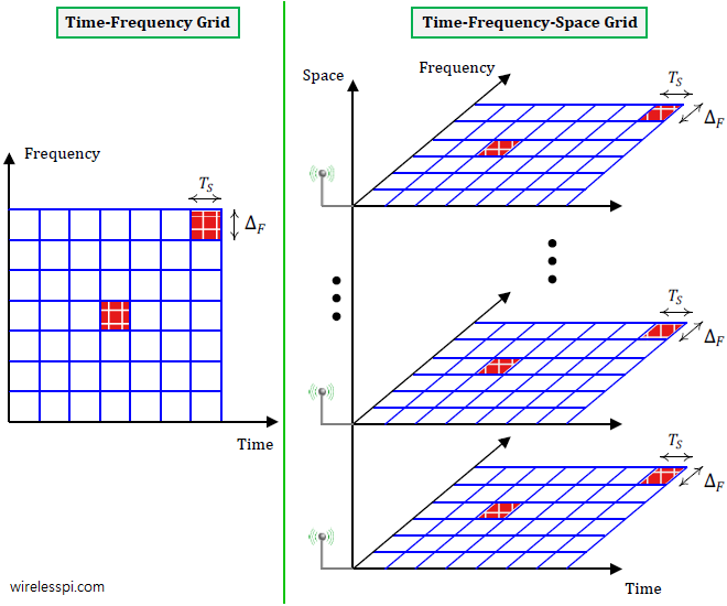
Time-Frequency Grid
Shown at the left of the figure below time-frequency grid where the available resources of time and frequency are sliced in discrete intervals. While the rise of digital computing made it straightforward to produce discrete time domain samples, the frequency part did not offer any such convenience. For most of the history of wireless communications, designers did not know how to slice the frequency domain at discrete points. This was due to the definition of frequency based on time itself, i.e., frequency is inversely proportional to time $T=1/F$. It was only after the formulation of Orthogonal Frequency Division Multiplexing (OFDM) technique that frequency domain could also be discretized in a convenient manner. This was one of the major reasons for adoption of OFDM systems in 4G and then 5G cellular standards.

Time-Frequency-Space Grid
Availability of multiple antennas on wireless devices adds another dimension to the resources at the disposal of the system designer. While frequency is dependent on time, there is no such limitation for space. Extra antennas can be utilized to sample additional versions of the same signal which can be exploited in a variety of manners. The right part of the above figure illustrates one time-frequency grid associated with each antenna. Consequently, instead of a time-frequency square as before, we have a time-frequency-space cube which can be employed for communication enhancement, reliability or directivity.