Mueller and Muller Timing Synchronization Algorithm

Proposed in 1976, Mueller and Muller algorithm is a timing synchronization technique that operates at symbol rate, as opposed to most other synchronization algorithms that require at least 2 samples/symbol such as early-late and Gardner timing error detectors. All of these are feedback techniques that operate within a PLL. Feedforward methods such as digital filter and square timing synchronization are also feasible due to powerful digital signal processing that avoids feedback problems such as hangups.

The most confusing thing communication engineers and radio hobbyists find about Mueller and Muller algorithm algorithm is the cross product in its expression: matched filter output at a symbol time is multiplied with the previous symbol value (instead of the symbol value at the same instant) and vice versa. I could not find any explanation for this confusion anywhere and that is the reason I wrote this post.

Before we start this topic, I recommend that you read about Pulse Amplitude Modulation (PAM) first due to two reasons.

• If you recently started learning about digital and wireless communication systems, it will give you an introduction to pulse amplitude modulated systems, the framework in which timing synchronization algorithms are described here.
• If you already know about communication receivers, the above post will introduce you to the notations I use for the system variables.

The notations for the main parameters are the following.

• Sample time (inverse of sample rate): $T_S$
• Symbol time (inverse of symbol rate): $T_M$
• Data symbols: $a[m]$
• Square-root Raised Cosine pulse shape: $p(nT_S)$
• Raised Cosine pulse shape: $r_p(nT_S)$ (as it is the auto-correlation of a Square-Root Raised Cosine pulse)
• Timing error: $\epsilon _\Delta$
• Timing error estimate: $\hat \epsilon _\Delta$

With these basics in place, we can now proceed towards an understanding of Mueller and Muller timing synchronization algorithm. There are two main kinds of Timing Error Detectors (TED) employed to achieve symbol timing synchronization through a PLL in a digital receiver:

• driving the derivative of the matched filter output to zero (such as a maximum likelihood TED, early-late gate TED)
• aligning one of the samples with zero crossings of the signal (such as a zero crossing TED, Gardner TED)

In both of these techniques, the maximum eye opening can be found at just $2$ samples per symbol. However, the final decision device (threshold detector) operates at the symbol rate, i.e., symbol-spaced samples of the matched filter output are required to generate symbol decisions.

On the other hand, we have already seen the detrimental effect of symbol rate sampling at $\epsilon _\Delta\neq 0$ in time and frequency domains. So here is the main question.

Can there be a timing error detector that successfully operates at this minimum rate of just $1$ sample/symbol?

The widely popular Mueller and Muller Timing Error Detector (TED) is one such example (probably someone with a sweet tooth later named it as M&M TED). Let us explore the intuition behind this algorithm.

Utilizing the Pulse Symmetry

---

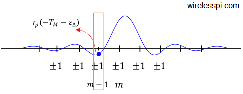
Figure below draws the impulse response of a pulse auto-correlation function, a Raised Cosine in this case. When the timing is almost right, i.e., $\epsilon _\Delta \approx 0$, then the two neighbouring samples taken before and after a symbol time $T_M$ should be almost equal. This is because when a sample is taken close to the peak of the pulse auto-correlation, all other symbol-spaced samples are near the zero crossings.

Mathematically, this can be written as
\begin{equation*}
r_p (+T_M-\epsilon _\Delta) \approx r_p (- T_M-\epsilon _\Delta)
\end{equation*}

and subsequently
\begin{equation}\label{eqTimingSyncMMRaisedCosine}
r_p (+T_M-\epsilon _\Delta) – r_p (- T_M-\epsilon _\Delta) ~\rightarrow~ 0
\end{equation}

From here, it seems that we need three samples to construct an expression for a timing error detector: one for the symbol value to remove the modulation and the other two for finding the slope. This also makes sense due to the samples being $+T_M$ and $-T_M$ away from the peak. However, Mueller and Muller devised a strategy that extracts the same information from two adjacent $T_M$-spaced samples.

The reasoning is quite simple: the relationship in Eq \eqref{eqTimingSyncMMRaisedCosine} is true only for timing offset $\epsilon _\Delta \approx 0$. As soon as $\epsilon _\Delta$ increases in magnitude, the asymmetry becomes visible. In the figure below for example, the right sample is larger than the left sample as $\epsilon _\Delta$ becomes more negative. The difference expression in Eq \eqref{eqTimingSyncMMRaisedCosine} then generates a timing error signal that is proportional to the actual timing offset $\epsilon _\Delta$. This error signal can be incorporated into a timing locked loop for the synchronization purpose.

Obtaining the error term

---

The question is how to obtain the two terms of the algorithm, i.e., $r_p (+T_M-\epsilon _\Delta)$ and $r_p (-T_M-\epsilon _\Delta)$, that are employed for the timing error detection. Imagine these two terms corresponding to the two seats of a seesaw (one near my home is shown below). This analogy is useful in understanding how the timing error detectors work because the crux of timing synchronization is all about balancing a seesaw.

We now refer to the figure below where symbol time $m$ is the reference. Here is the interesting reasoning behind how the algorithm works.

• Generating $r_p (+T_M-\epsilon _\Delta)$: Since the samples are symbol-spaced, their values are close to $\pm 1$ in steady state. Any kind of summation tends all the samples towards zero. The matched filter output $z(mT_M)$ is made up of contributions from symbol $m$ and all the neighbouring symbols. From symbol $m-1$, the pulse autocorrelation $r_p(nT_S)$ brings a value $r_p(+T_M-\epsilon _\Delta)$ at time $m$ that is one symbol into the future. If we multiply $z(mT_M)$ with $a[m-1]$, this removes the modulation of symbol $m-1$ and only the term $r_p(+T_M-\epsilon _\Delta)$ adds up coherently each time. This is drawn in the figure below.



• Generating $r_p (-T_M-\epsilon _\Delta)$: From symbol $m$, the pulse autocorrelation $r_p(nT_S)$ sends a value $r_p(-T_M-\epsilon _\Delta)$ back at symbol time $m-1$ that is one symbol into the past. Multiplying the matched filter output $z((m-1)T_M)$ with $a[m]$ removes the modulation of symbol $m$ and produces only $r_p(-T_M-\epsilon _\Delta)$. This is shown in the figure below.

Next, we translate the above findings into a more formal expression. First, the ideal transmitted signal is written as
\begin{equation*}
s(nT_S) = \sum \limits _i a[i] p(nT_S – iT_M)
\end{equation*}

where $a[i]$ are the modulation symbols, $p(nT_S)$ is the Square-Root Nyquist pulse while $T_S$ and $T_M$ are sample and symbol times, respectively. This signal received with a timing delay $\epsilon_\Delta$ is given by

\begin{equation*}
r(nT_S) = \sum \limits _i a[i] p(nT_S – iT_M-\epsilon _\Delta)
\end{equation*}

At the receiver, the matched filter output is written as
\begin{align*}
z(nT_S) &= r(nT_S) * p(-nT_S) \\
&= \Big\{ \sum \limits _i a[i] p(nT_S – iT_M-\epsilon _\Delta)\Big\} * p(-nT_S) \\
&= \sum \limits _i a[i] r_p(nT_S -iT_M -\epsilon _\Delta)
\end{align*}

For an initial timing estimate $\hat \epsilon _\Delta = 0$, sampling at $n = mL = mT_M/T_S$ produces the output at $L=1$ sample/symbol as
\begin{align*}
z(mT_M) &= \sum \limits _i a[i] r_p (mT_M – iT_M – \epsilon _\Delta) \\
&= \sum \limits _i a[i] r_p \big\{(m-i)T_M – \epsilon _\Delta \big\}
\end{align*}

Next, recall that for a binary PAM, the data symbols take values from a finite symbol set $\{-1, +1\}$. Each such option has a $1/2$ chance of occurring, hence whenever $i\neq m$, the average of $a[m]\cdot a[i]$ is zero, otherwise it is equal to $1$ for $i=m$.
\begin{equation*}
\text{Mean}\{a[m]\cdot a[i]\} =
\begin{cases}
1 & \quad i = m \\
0 & \quad \text{otherwise}
\end{cases}
\end{equation*}

In the light of the above, let us evaluate the following expression.
\begin{equation*}
\text{Mean}\left\{a[m-1]\cdot z(mT_M)\right\} = \text{Mean} \left\{ a[m-1]\cdot \sum \limits _i a[i] r_p \big\{(m-i)T_M – \epsilon _\Delta \big\}\right\}
\end{equation*}
Only for $i=m-1$, the above average is non-zero. Therefore, plugging $i=m-1$ in the above expression,
\begin{equation*}
\text{Mean}\left\{a[m-1]\cdot z(mT_M)\right\} = 1\cdot r_p (+T_M – \epsilon _\Delta ) = r_p (+T_M – \epsilon _\Delta )
\end{equation*}

Using a similar logic by plugging $i=m$ above,
\begin{align}
\text{Mean}\left\{a[m]\cdot z((m-1)T_M)\right\} &= \nonumber\\
&\hspace{-.8in}\text{Mean} \left\{ a[m]\cdot \sum \limits _i a[i] r_p \big\{(m-1-i)T_M – \epsilon _\Delta \big\}\right\} \nonumber\\
&= r_p(-T_M – \epsilon _\Delta) \label{eqTimingSyncMM2}
\end{align}

Comparing the above two expressions with the basic principle behind balancing the matched filter output in Eq \eqref{eqTimingSyncMMRaisedCosine}, it can be seen that
\begin{equation*}
r_p (+T_M-\epsilon _\Delta) – r_p (- T_M-\epsilon _\Delta) = a[m-1]z(mT_M) – a[m]z((m-1)T_M)
\end{equation*}

With our usual notation of sampling at a phase $\hat \epsilon _\Delta$, a timing error detector can be constructed as
\begin{equation}\label{eqTimingSyncMMTEDDA}
e_D[m] = a[m-1] z(mT_M+\hat \epsilon _\Delta) – a[m]z((m-1)T_M+\hat \epsilon _\Delta)
\end{equation}

This is the data-aided version of Mueller and Muller TED. For a decision-directed representation, the symbols $a[m]$ are replaced with their estimates $\hat a[m]$ as
\begin{equation*}
e_D[m] = \hat a[m-1]z(mT_M+\hat \epsilon _\Delta) – \hat a[m]z((m-1)T_M+ \hat \epsilon _\Delta)
\end{equation*}

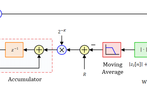
A block diagram for the implementation of an M&M TED is shown in the figure below where the symbol $T_M$ denotes a delay of a symbol time.

Let us explore its implementation in GNU Radio.

GNU Radio Block: Clock Recovery MM

---

The block Clock Recovery MM implements an M&M TED with the following parameters. Keep in mind that all timing synchronization blocks in GNU Radio will eventually become a part of the symbol synchronization block written by Andy Wells.

• Omega: This is our initial estimate of the number of samples/symbol $L$. In the presence of a Sampling Clock Offset (SCO), the actual value is slightly different and is unknown but it can nevertheless be set to $L$.
• Gain Omega: This is the gain setting for the Integrator constant $K_i$ of a Proportional + Integrator (PI) loop filter as explained in the article on phase locked loops. You should set this value as
  \begin{equation*}
  \text{`Gain Omega’} = \frac{\text{`Gain Mu’}^2}{4}
  \end{equation*}
  where `Gain Mu’ is the proportional gain $K_p$, see below.
• Mu: This is our initial guess of the timing phase offset $\epsilon _\Delta$. While an initial estimate $L$ of Omega above is reasonably close to the actual value, it is impossible to guess $\epsilon _\Delta$ in advance. Therefore, it is best to set this value equal to $0.5$ with the implicit assumption that $\epsilon _\Delta$ is uniformly distributed between $0$ and $1$.
• Gain Mu: This is the proportional part $K_p$ of the PI loop filter. Now the reason M&M clock recovery is considered as a confusing block is that it is only the loop bandwidth that is required in many other synchronization blocks while here the input is directly $K_p$ and $K_i$ (also called `alpha’ and `beta’, respectively) of the loop filter. How to set this value requires some derivation which is explained in my book.
• Omega Relative Limit: This sets the maximum relative deviation from Omega above and depends on the clock specifications, i.e., ppm rating.

You can think of this implementation of M&M TED in GNU Radio as explicitly correcting both the timing phase offset $\epsilon _\Delta$ as well as the sampling clock offset. If a signal is sampled at time $mT_M$, then the subsequent sample time in an ideal case is $mT_M$ $+$ $T_M$. In current GNU Radio implementation, a slowly changing symbol time is injected to mitigate the sampling clock offset as
\begin{align*}
\text{Updated symbol time} &= \text{Previous symbol time} + (\text{`Gain Omega’})e_D[m]\\
\text{Updated symbol phase} &= \text{Previous symbol phase} + \text{Updated symbol time} + \\
&\hspace{2.3in}(\text{`Gain Mu’}) e_D[m]
\end{align*}
where the expression `symbol phase’ refers to the timing phase and not a carrier phase. If we run an M&M clock recovery block in GNU Radio choosing the default values for the above parameters as $K_p=0.175$ and $K_i=K_p^2/4$ for a $16$-QAM scheme with excess bandwidth $\alpha=0.1$ and $L=4$ samples/symbol, figure below plots the input and output constellations.

A final word of caution: since the M&M TED does not involve any cancellation of phase through a conjugate product, it is not carrier independent and thus more suitable for timing synchronization after the settling of carrier loops in a steady state tracking mode.