In the article on Zero-Forcing detector for MIMO receivers, we have seen that the performance of linear detectors is unsatisfactory for actual implementations of conventional MIMO systems. Their main attraction comes from their low computational complexity. To strike a nice balance between performance and complexity, a neat trick is employed by the algorithm known as Successive Interference Cancelation (SIC). The concept was devised by Gerard Foschini from Bell Labs, although it was not a new idea. Successive interference cancelation was already proposed for the detection algorithms in CDMA systems. Again, the fundamental idea was borrowed from decision feedback equalization schemes in single-carrier systems. Owing to the analogy between interference among different CDMA users and multiple Tx antenna streams, the same algorithm was tweaked in the context of MIMO detection.
We first reproduce the system architecture first.
Spatial Multiplexing
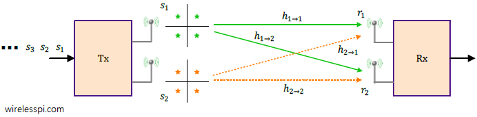
A block diagram for a multiple antenna system with $N_T$ Tx antennas and $N_R$ Rx antennas is drawn in the figure below. In this spatial multiplexing mode, separate bits modulated as $s_1$, $s_2$, $\cdots$, $s_{N_T}$, are simultaneously sent through their respective Tx antennas. For example, for $N_T=2$, the first antenna sends $s_1$, $s_3$, $s_5$, $\cdots$ while the second antenna transmits $s_2$, $s_4$, $s_6$, $\cdots$.

The channel gain between $i$-th Tx antenna and $j$-th Rx antenna is denoted by $h_{(i\rightarrow j)}$. Observe on the Rx side of the above figure that the cumulative signal at each antenna is a summation of signals arriving from all Tx antennas.
$$\begin{equation}
\begin{aligned}
r_j = h_{(1\rightarrow j)}\cdot s_1 + h_{(2\rightarrow j)}\cdot s_2 + \cdots + h_{(N_T\rightarrow j)}\cdot s_{N_T} + \text{noise}, \qquad \\
\qquad j = 1, 2, \cdots,N_R
\end{aligned}
\end{equation}\label{equation-sp-general}$$
These equations can be written into a matrix form as
\begin{equation}\label{equation-r-matrix}
\mathbf{r=H\cdot s+\text{noise}}
\end{equation}
where
- $\mathbf{r}$ is a vector consisting of elements $r_j$, i.e., the signals arriving at Rx antennas
- $\mathbf{s}$ is a vector consisting of the modulation symbols $s_i$
- $\mathbf{H}$ is a matrix of channel coefficients
Since the signals from all Tx antennas arrive at each Rx antenna, the main task of the detection algorithms here is to free each modulated bit sent by one Tx antenna from the interference of the other modulated bits sent by rest of the Tx antennas. Today, we describe the most commonly used linear algorithm, known as Zero-Forcing (ZF), to accomplish this task.
Vertical-Bell Laboratories Layered Space-Time (V-BLAST)
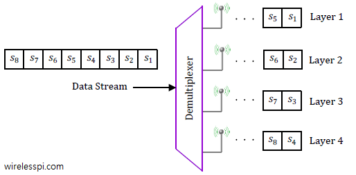
On the Tx side, the mapping architecture was named as V-BLAST which stands for Vertical-Bell Laboratories Layered Space-Time architecture (the term layer originates from the spatial streams in Tx antennas). The term V-BLAST stems from the fact that modulation symbols $s_1$, $s_2$, $\cdots$, are presented to the Tx antennas in order from $1$ to $N_T$. An example for $N_T=4$ antennas is illustrated in the figure below where the binary data is coded and modulated first and then a demultiplexer maps successive symbols to respective antennas. In the figure, for instance, symbol $s_1$ is mapped to the first antenna, $s_2$ to the second antenna and so on. This cycle continues forming data layers in space until the symbol $s_5$ comes back to Tx antenna 1. V-BLAST is a different architecture as compared to Diagonal or D-BLAST in which coded modulation symbols are presented to Tx antennas in a cyclical manner. This makes each stream or layer being sent in a diagonal of space and time thus increasing the reliability.

On the Rx side, a Successive Interference Cancellation (SIC) algorithm is employed. Despite this fancy name, the underlying concept is quite easy. Let us first explain an intuitive sense of its operation.
- First, multiple spatial streams or layers are put in a descending ordered based on some chosen criterion (e.g., highest SNR stream first).
- Next, a linear detection algorithm like Zero-Forcing or MMSE that have been discussed before is applied to detect the modulation symbols of the first stream.
- Since the channel gains are known at the Rx, the full impact of this stream or layer can then be removed by subtraction from the received signal! In case the decisions were correct, the new signal now contains contributions from $N_T-1$ spatial streams but not from the first one. This again allows the detection of the second layer in order through a linear algorithm.
- The process is continued until the last spatial stream is estimated.
Now we turn towards the actual implementation details with an example of a 2×2 MIMO system, i.e., $N_T=2$ and $N_R=2$ as shown in the figure below.
The system model is reproduced here from the article on linear detectors.
\begin{equation}\label{equation-sp-2×2-again}
\begin{aligned}
r_1 &= h_{(1\rightarrow 1)}\cdot s_1 + h_{(2\rightarrow 1)}\cdot s_2 + \text{noise} \\
r_2 &= h_{(1\rightarrow 2)}\cdot s_1 + h_{(2\rightarrow 2)}\cdot s_2 + \text{noise}
\end{aligned}
\end{equation}
Now refer to the flowchart in the figure below showing the ordered successive interference cancellation algorithm to understand what follows.

Ordering and First Stream Detection
This method starts with the ordering of the two streams according to some chosen criterion (e.g., SNR). Then, a linear detection algorithm (e.g., Zero-Forcing or MMSE) can be applied to detect the modulation symbols from the first stream as derived here.
\[
\hat s_1 = \frac{h_{(2\rightarrow 2)}\cdot r_1 – h_{(2\rightarrow 1)}\cdot r_2}{h_{(2\rightarrow 2)}\cdot h_{(1\rightarrow 1)} – h_{(2\rightarrow 1)}\cdot h_{(1\rightarrow 2)}}
\]
This brings us to the next stage.
Removal of Interference
Having known the first stream and assuming the decisions were correct, its impact can be removed from all the Rx signals through subtraction. Assuming that $\hat s_1$ was detected, Eq (\ref{equation-sp-2×2-again}) is modified as
$$\begin{equation}
\begin{aligned}
\tilde{r}_1 ~~=~~ r_1 – h_{(1\rightarrow 1)}\cdot \hat s_1 ~~&=~~ \require{cancel}\cancelto{0}{h_{(1\rightarrow 1)}\cdot \Big\{s_1-\hat s_1\Big\}} \quad+ h_{(2\rightarrow 1)}\cdot s_2 + \text{noise} \\
\tilde{r}_2 ~~=~~ r_2 – h_{(1\rightarrow 2)} \cdot \hat s_1 ~~&=~~ \require{cancel}\cancelto{0}{h_{(1\rightarrow 2)}\cdot \Big\{s_1 – \hat s_1\Big\}} \quad+ h_{(2\rightarrow 2)}\cdot s_2 + \text{noise}
\end{aligned}
\end{equation}\label{equation-sic-s2}$$
If there are no errors, i.e., $\hat s_1=s_1$, the contribution from $s_1$ cancels out at both Rx antennas! In case there are more than $2$ spatial streams, then the linear algorithm can be applied again to detect $s_2$. Subsequently, the interference contribution from $s_2$ can be removed by subtraction in a similar manner as shown above for $s_1$.
Detection of Last Stream
Observe that the signals $\tilde{r}_1$ and $\tilde{r}_2$ above have become functions of modulation symbol $s_2$ only. We have two independent equations and one unknown. In case of a single layer or a single antenna system, there is no difference between Maximum Ratio Combining (MRC) and a Zero-Forcing solution. So the same algorithm can be applied to estimate $\hat s_2$ which looks like MRC technique. This incorporates the SNR from all the Rx antennas and hence the weights $w_i$ should be conjugates of complex channel gains involved with $s_2$ in Eq (\ref{equation-sic-s2}).
\[
h_{(2\rightarrow 1)}^*\cdot \tilde{r_1} + h_{(2\rightarrow 2)}^*\cdot \tilde{r_2} = \Big\{ |h_{(2\rightarrow 1)}|^2+|h_{(2\rightarrow 2)}|^2\Big\} \cdot s_2 + \text{noise}
\]
The decision on $s_2$ can now be taken as the constellation point closest to the value from the left hand side above.
\[
\hat s_2 = \frac{h_{(2\rightarrow 1)}^*\cdot \tilde{r_1} + h_{(2\rightarrow 2)}^*\cdot \tilde{r_2}}{|h_{(2\rightarrow 1)}|^2+|h_{(2\rightarrow 2)}|^2}
\]
To help the reader understand the idea, observe that the figure above is drawn with a hidden RGB (Red, Green, Blue) coloring scheme. Since white color contains an equal contribution from all of them, the signal input to the algorithm is shown as white in color. After the blue stream is detected, the arrows are shown as blue while the Zero-Forcing is applied now to a combination of Red and Green, i..e, yellow. After the detection of Green layer, the arrows are green and the final Red stream is detected in the end. The last box for stream $N_T$ is drawn black since black color means absence of all colors.
A few comments regarding this scheme are in order.
Diversity order: A linear algorithm is applied for the detection of the first spatial stream ($s_1$ in our example above). Consequently, the diversity order is similar to what we found for linear detection of the previous section: $N_R-N_T+1$. However, as compared to the detection of $s_1$, one spatial stream $s_2$ next is detected through two Rx antennas, see Eq (\ref{equation-sic-s2}). This is similar to the scenario of $1$ Tx antenna and $2$ Rx antennas. Therefore, the diversity order for $s_2$ is $2$.
The advantage of this scheme is now clear. The modulation symbols that are detected successively at later stages benefit from a progressively higher diversity order. Consequently, the diversity order is equal to $N_R$ for the last stream because that is virtually detected with $N_R$ antennas at the Rx.
Error Propagation: Notice from Eq (\ref{equation-sic-s2}) that the terms involving $s_1-\hat s_1$ only go to zero if $\hat s_1$ $=$ $s_1$. Otherwise, instead of removing the interference, such an operation actually injects more interference into the output streams thus making it more difficult to detect the modulation symbols down the subsequent stages. This is known as error propagation.
Ordering: Due to error propagation, the order in which streams are chosen for estimation and subsequent interference removal significantly impacts the overall performance. There are different methods for this purpose such as SNR based ordering, Signal to Interference plus Noise (SINR) based ordering and ordering based on channel gains of each particular stream (e.g., $h_{(1\rightarrow 1)}$, $h_{(2\rightarrow 1)}$, $\cdots$, $h_{N_T \rightarrow 1}$ all belong to symbol $s_1$).
Finally, some other non-linear algorithms like maximum likelihood detection outperform successive interference cancelation at a cost of higher computational complexity.