We have seen before how a symbol timing offset severely impacts the constellation of the received symbols. Therefore, symbol timing recovery is one of the most crucial jobs of a digital communications receiver. In the days of analog clock recovery, a timing error detector provided the instant to sample the Rx waveform at 1 sample/symbol at the maximum eye opening. However, discrete-time processing opened the doors for better timing recovery schemes as an ever increasing number of transistors within the same area consistently keeps bringing the digital processing cost down. Consequently, the use of analog circuits to control the timing were not economically feasible anymore and methods from digital processing gradually became the norm. Everything that was implemented by real circuit elements got replaced with the lines of code in a microprocessor that perform the same operations right out of the pure mathematical equations.
For this purpose, there are two main approaches: feedback and feedforward.
- In the feedback approach, timing error detectors such as maximum likelihood, early-late, zero-crossing and Mueller and Muller are employed in a Phase Locked Loop (PLL).
- In the feedforward approach, a direct estimate of the timing offset is generated which is the topic of discussion in this article.
Background
For a digital modem where digital signal processing techniques are applied to an already sampled signal, a direct estimate of the symbol timing offset $\hat \epsilon_{\Delta}$ can be obtained as follows. The notations for the main parameters are the following.
- Sample time (inverse of sample rate): $T_S$
- Symbol time (inverse of symbol rate): $T_M$
- Data symbols: $a[m]$
- Square-root Raised Cosine pulse shape: $p(nT_S)$
- Raised Cosine pulse shape: $r_p(nT_S)$ (as it is the auto-correlation of a Square-Root Raised Cosine pulse)
- Timing error: $\epsilon _\Delta$
- Timing error estimate: $\hat \epsilon _\Delta$
Now assume that the Rx signal is sampled at a rate of $F_S = 1/T_S = L/T_M$ where $T_M$ is the symbol time and $L$ is the oversampling factor, or samples/symbol.
\begin{equation*}
r(nT_S) = \sum _m a[m] p(nT_S-mT_M-\epsilon_{\Delta})
\end{equation*}
Here, $p(nT_S)$ is a square-root Nyquist pulse such as a Square-Root Raised Cosine. The spectral line after squaring appears at $\pm 1/T_M$ because squaring in time domain is convolution of the signal with itself in frequency domain, hence doubling the bandwidth. Consequently, the parameter $L$ should be chosen according to the sampling theorem, i.e., more than twice the highest frequency component of the input signal, i.e.,
\begin{equation*}
F_S = \frac{L}{T_M} > 2\cdot \frac{1}{T_M} \qquad \Rightarrow \qquad L > 2
\end{equation*}
For this reason, $L$ must be an integer greater than $2$. It is a common practice to choose $L=4$ for this purpose due to a simple estimator architecture, as we shortly see.
After converting the signal into digital domain, it is matched filtered with a similar but flipped pulse shape $p(-nT_S)$. That accounts for the digital filter part in the name of this scheme.
\begin{align*}
z(nT_S) &= r(nT_S) * p(-nT_S) \\
&= \Big\{\sum \limits _m a[m] p(nT_S – mT_M-\epsilon_{\Delta})\Big\} * p(-nT_S) \\
&= \sum \limits _m a[m] r_p(nT_S – mT_M-\epsilon_{\Delta})
\end{align*}
where $r_p(nT_S)$ is the Nyquist pulse such as a Raised Cosine. Since the sample rate is chosen large enough, no information is lost in digital transformation and squaring the digital signal produces the same timing lines, which is the reason the name digital filter and square timing recovery.
Timing Estimate
To locate this spectral line, we take the Discrete Fourier Transform (DFT) of the squared signal (see Chapter 7 of my wireless communications book for the intuitive reasoning behind why almost all timing recovery techniques are derived from squaring the modulated signal).
\begin{equation*}
Y[k] = \text{DFT}~|z(nT_S)|^2
\end{equation*}
Exploiting the fact that $|z(nT_S)|^2$ is a real signal with zero $Q$ component, the DFT definition yields
\begin{align}\label{eqTimingSyncSquareDFT}
Y_I[k]\: &= \sum \limits _{n=0} ^{N-1} |z(nT_S)|^2 \cos 2\pi\frac{k}{N}n\\
Y_Q[k] &= -\sum \limits _{n=0} ^{N-1} |z(nT_S)|^2 \sin 2\pi\frac{k}{N}n
\end{align}
However, all DFT components $k=-N/2,\cdots,-1,0,1,\cdots, N/2-1$ of the sequence are not required because the matched filter output is bandlimited to $(1+\alpha)/2T_M$ while the squared signal due to convolution in frequency domain is bandlimited to
\begin{equation*}
B_{|z(nT_S)|^2} = \frac{1+\alpha}{T_M} \le \frac{2}{T_M}
\end{equation*}
Consequently, only the DFT component corresponding to $F=\pm 1/T_M$ should be enough for timing purpose. So instead of computing the full DFT, only a single such component can be calculated if its position $k$ is known. Now we exploit one of the most useful relations to travel between discrete and continuous frequencies $k/N=F/F_S$. This gives the timing lines at the following discrete frequencies.
\begin{equation*}
\pm \frac{F}{F_S} = \pm \frac{1/T_M}{1/T_S} = \pm \frac{1/(LT_S)}{T_S} = \pm \frac{1}{L}
\end{equation*}
Assume that a data packet contains a total of $N_d$ symbols. Ignoring the group delay $G$ on either side of the matched filtered and squared signal, the length of the sequence is $N=L\cdot N_d$. Since the above expression $F/F_S$ is equal to $k/N$, we get
\begin{equation*}
\frac{k}{N} = \pm \frac{1}{L} \quad \rightarrow \quad k = \pm N_d
\end{equation*}
This is the DFT component corresponding to our spectral line. Consequently, we plug it into DFT Eq (\ref{eqTimingSyncSquareDFT}) above.
\begin{align*}
Y_I[N_d]\: &= \sum \limits _{n=0} ^{N-1} |z(nT_S)|^2 \cos 2\pi\frac{N_d}{N}n\\
Y_Q[N_d] &= -\sum \limits _{n=0} ^{N-1} |z(nT_S)|^2 \sin 2\pi\frac{N_d}{N}n
\end{align*}
By using $N=L\cdot N_d$,
\begin{align}\label{eqTimingSyncL4}
Y_I[N_d]\: &= \sum \limits _{n=0} ^{N-1} |z(nT_S)|^2 \cos 2\pi\frac{1}{L}n\\
Y_Q[N_d] &= -\sum \limits _{n=0} ^{N-1} |z(nT_S)|^2 \sin 2\pi\frac{1}{L}n
\end{align}
Recall that the phase of this spectral component produces our estimate of timing delay and a delay in time manifests itself as sinusoidal phase, i.e., a rotation of spectral impulses.
\begin{equation}\label{eqTimingSyncFilterSquareEstimate}
\hat \epsilon_{\Delta} = -\frac{1}{2\pi} \measuredangle Y[N_d]
\end{equation}
To avoid an extra phase term from the asymmetrical summation from $n=0$ to $N-1$, a symmetrical sum from $n=-N/2$ to $N/2-1$ can also be taken. The above expression seems to be a remarkable result since it generates a timing estimate from a phase estimate! Looking back, this is not a surprise.
Implementation
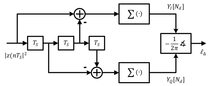
As you might have noticed, we have skipped some mathematical details to rigorously derive the above estimator. The above estimator requires at least $L=4$ samples/symbol and feedforward solutions have been proposed to reduce it to $L=2$ samples/symbol at the cost of extra complexity. Observe from Eq (\ref{eqTimingSyncL4}) that for this particular value of $L$ equal to $4$, the cosine and sine decompose into following simple relations.
\begin{align*}
\cos \frac{2\pi}{4}n &= \cos \frac{\pi}{2}n = ~1,~0,\:-1,~0,\cdots \\
\sin \frac{2\pi}{4}n &= \sin \frac{\pi}{2}n = ~0,~1,~0,\:-1,\cdots
\end{align*}
The main attraction of this choice is that a multiplication-free realization of the timing estimator is obtained, a block diagram of which is drawn in the figure below with $T_S$ representing one sample delay. Match the negative signs of the cosine and sine above with those in the block diagram. The negative signs in the $Q$ arm are inverted due to the negative sign in Eq (\ref{eqTimingSyncL4}).

As far as the discussion above is concerned, this estimate can be utilized for timing recovery in a short packet. For other scenarios, emulating an analog approach of reconstructing a digital symbol rate clock is not our purpose and instead we want to know where the optimal sampling instant corresponding to the maximum eye opening during each symbol is located. This can be done in a very simple manner with just $L=2$ or even $L=1$ sample/symbol, for which we can design a feedback solution by utilizing the insights developed through the squaring approach. Some of these examples are early-late, zero-crossing or Gardner and Mueller and Muller timing error detectors.


Nice explanation Qasim.
I was wondering if this method will still work if the pulse shape is rectangular (not raised cosine)? These pulses are used in optical noncoherent communication.
Thanks. For a rectangular pulse, the squared version is the same and the spectrum is a sinc. There is no concept of excess bandwidth in that case and hence no spectral impulses are generated at symbol rate. An early-late timing recovery is one feasible option.
Hey Qasim,
Thank you for this great explanation. I am wondering about the output of the timing recovery. After the signal is resampled at the maximum eye opening, we are still left with 4 samples / symbol. How would we determine which is the best to take? The PLL structures all seem to be focused on 1 or 2 samples/symbol.
Thank you!
Timing recovery chain uses 4 samples/symbol here, not the signal demodulation that can downsample the signal as desired. Once the frame sync block delivers the first symbol and timing recovery block delivers the timing phase, the exact sample for demodulation can be known.
Hi Qasim,
Thanks for the nice explanation. Could you please elaborate why we are in particular interested in the spectral component at frequency 1/Tm?
Thanks!
A digitally modulated signal represents an underlying cyclostationary random process with period $T_M$. The autocorrelation function has spectral components at integer multiples of symbol rate $1/T_M$. But the pulse shape limits the bandwidth and hence all components beyond $1/T_M$ are gone. We are left with only 1 symbol rate spectral line.
Hi Qasim,
It has been a nice explanation of very interesting topic. Just wondering if it’s better to place a pulse shaping filter on a receiver side before a correlator or after a correlator in case of simple correlation receiver?
Provided we still have two samples per symbol for correlation even after a pulse shaping filter (offering down sampling as well)
Thanks
Hi Saqib, thanks. I’m trying to understand your question. If your receiver has a pulse shaping filter which is a matched filter, then it performs correlation as well by definition, see the difference between correlation and matched filtering here.
If you’re looking for the location of shaping filter in the receiver, this explanation might help.