In Maximum Ratio Combination (MRC), our focus was on combining the signals from multiple antennas at the Rx side. Here, we will see how a similar system can be developed with multiple antennas at the Tx side.
As our first consideration, we attempt to replicate the results of Rx diversity in a scenario where there are multiple Tx antennas and a single Rx antenna. This is commonly known as a Multiple-Input Single Output (MISO) system. Assume that there are $N_T$ Tx antennas available and only a single Rx antenna as shown in the figure below. This is a dual problem of 1 Tx antenna and multiple Rx antennas.

- Since our focus is on one symbol, we can temporarily remove the time index $m$ and denote the data symbol by $s$ only.
- At this stage, no knowledge about the channel gains is assumed at the Tx. Therefore, the power is equally divided among the two antennas and hence amplitude of the signal (which is the square root of power) is given by $1/\sqrt{2}$.
- Each Tx antenna emits the same signal which encounters the flat fading channel gain $h_j$ on its way to the Rx.
Now the nature adds the signals impinging at the single Rx antenna allowing us to write
\begin{equation}\label{equation-miso-1}
\begin{aligned}
r &= h_1\cdot \frac{s}{\sqrt{2}} + h_2\cdot \frac{s}{\sqrt{2}} + \text{noise} = \underbrace{\frac{h_1+h_2}{\sqrt{2}}}_{h}s + \text{noise} \\
&= h\cdot s + \text{noise}
\end{aligned}
\end{equation}
As explained before, the channel gains $h_1$ and $h_2$ are complex Gaussian random variables with uniformly distributed phases between $0$ and $2\pi$. Their sum also follows a Gaussian distribution with a uniform phase and adding several complex numbers with random phases tends to average out the summation! The conclusion is that there is no diversity gain in this setup.
To do better, the trick is to copy the same architecture employed for MRC before but reverse the roles of antennas if the channel knowledge is available at the Tx. The resulting technique is known as Maximum Ratio Transmission (MRT) (this term is also used for maximizing diversity reception through linear precoding when both the Tx and the Rx are equipped with multiple antennas. I choose the more common and simpler use of the terminology here for ease of understanding). A block diagram of this scheme for 2 Tx antennas and 1 Rx antenna is drawn in the figure below, a dual of the MRC block diagram at the Rx. Here, the modulation symbol $s$ is weighted by $w_1$ and $w_2$ before sending it through the first and second Tx antennas, respectively. Nature adds these signals at the Rx antenna and the result can be expressed as
\[
\begin{aligned}
r &= w_1\cdot h_1\cdot s + w_2\cdot h_2\cdot s+ \text{noise} \\
&= s\cdot \left\{w_1\cdot h_1+w_2\cdot h_2\right\} + \text{noise}
\end{aligned}
\]

This is exactly the same equation as encountered for MRC at the Rx before and hence the same analysis can be applied here. Consequently, if we choose random and fixed $w_i$, their sum would neither cancel the phases nor grade the magnitudes. Instead, the modulation symbol $s$ must be weighted by $w_i$ in each branch such that the natural summation at Rx antenna coherently adds electromagnetic energy emanating from each Tx antenna. This can be accomplished by implementing the same solution as in the case of MRC at the Rx, i.e., optimal weights $w_i$ are complex conjugates of channel gains $h_i$.
\begin{equation}\label{equation-weights-mrc-tx-1}
w_i = h^*_i
\end{equation}
where I have again ignored the scaling factor $1/\sqrt{\sum \nolimits_{i=1}^{N_T} |h_i|^2}$ to keep the expressions simple. When optimal $w_i$ are chosen, the signal at the Rx antenna becomes
\begin{equation}\label{equation-weights-mrc-tx-2}
r = \left\{h_1^*\cdot h_1+h_2^*\cdot h_2\right\}\cdot s + \text{noise} = \Big\{ |h_1|^2+|h_2|^2\Big\}\cdot s + \text{noise}
\end{equation}
which we found in MRC scenario at the Rx as well. The improvement lies in the multiplicative factor with the modulation symbol $s$. Previously it was a fading coefficient $h$ that was the sum of $h_1$ and $h_2$ that could potentially bring each other down. Now the factor appearing with data symbol $s$ is $|h_1|^2+|h_2|^2$. Here, not only that the contribution from each channel gain $h_i$ is taken according to its own energy but also the magnitude squared operation completely cancels the phase for each $h_i$. This is the best we can do in focusing the energy towards the intended destination.
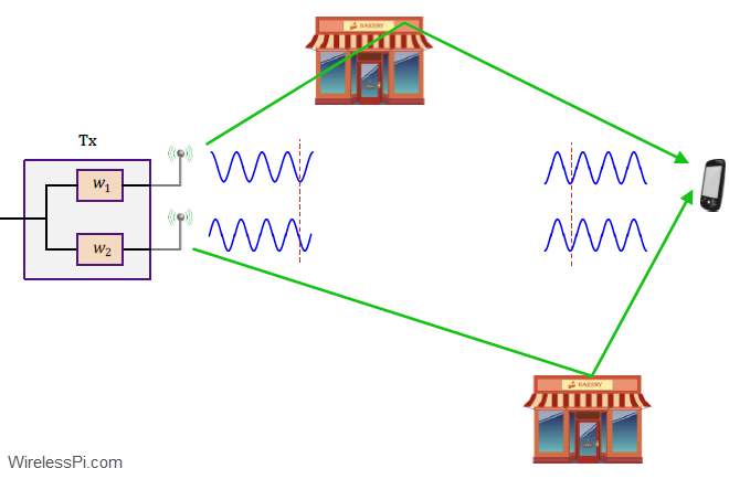
To get an intuitive sense of how this choice works at the Tx side, an example of a simple manipulation is drawn in the figure below. Without any weighting at the Tx, the two signals from both antennas will mostly cancel each other at the Rx. However, utilizing the channel knowledge, the Tx adjusts its phase at second antenna before the transmission such that signals from both antennas now arrive at the Rx in phase with each other. In 5G systems with a large number of base station antennas and a simple user terminal, this is how beamforming is implemented in non-LoS scenarios.