Zero-Forcing (ZF) Detection in Massive MIMO Systems

Massive MIMO is one of the defining technologies in 5G cellular systems. In a previous article, we have described spatial matched filtering (or maximum ratio) as the simplest algorithm for signal detection. Here, we explain another linear technique, known as Zero-Forcing (ZF), for this purpose. It was described before in the context of simple MIMO systems here.

Background

---

Consider the block diagram for uplink of a massive MIMO system as drawn below with $N_B$ base station antennas and $K$ mobiler terminals.

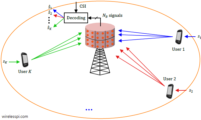
It is evident that the cumulative signal at each base station antenna $j$ is a summation of signals arriving from each user terminal $i$. While the expression below looks complicated, observe from the figure that the signal at each antenna is simply a sum of individual modulation symbols $s_1$, $s_2$, $\cdots$, $s_K$ scaled by channel coefficients.
$$\begin{equation}
\begin{aligned}
r_j = h_{(1\rightarrow j)}\cdot s_1 + h_{(2\rightarrow j)}\cdot s_2 + \cdots + h_{(K\rightarrow j)}\cdot s_{K} +~&~ \text{noise}, \qquad \\
& \qquad j = 1, 2, \cdots,N_B
\end{aligned}
\end{equation}\label{equation-massive-mimo-detection}$$

Here, the flat fading channel gain between $i$-th user terminal ($i=1,2\cdots,K$) and $j$-th base station antenna ($j=1,2,\cdots,N_B$) is denoted by $h_{(i\rightarrow j)}$. Power control is ignored here for simplicity. The reader should keep in mind that power control is important in cellular systems to prevent signals from users with strong channels drowning the signals coming from weak users. However, power control coefficients depend on large-scaling fading that renders them independent of both frequency and fast update rates.

Eq (\ref{equation-massive-mimo-detection}) tells us that the original signal received at the base station is not coming from terminal 1 alone! Instead, all user terminals transmit simultaneously on the uplink and hence the cumulative signal $r_j$ at each antenna $j$ is a superposition of signals from $K$ terminals. As a result, interference from $K-1$ users is added to the desired signal. The main task of the detection algorithms here is to free each modulation symbol $s_i$ sent by a user terminal $i$ from the interference of the other modulation symbols sent by rest of the mobile users.

If maximum ratio or spatial matched filtering is applied to solve this problem, the favorable propagation scenario is approximately true and the relation is not exact. Hence, low amounts of interference from other terminals can still leak into the desired signal causing a degradation in performance. Our goal here is to make up for that performance loss without incurring significant computational complexity. Zero-Forcing (ZF) algorithm provides that solution which is slightly more complex than matched filtering but compensates for the performance loss at the same time.

A proper derivation of Zero-Forcing solution requires dealing with matrices since $K$ user terminals communicate with $N_B$ base station antennas on the uplink. All that data combined results in an $N_B$ $\times$ $K$ matrix of channel gains. However, I will present a simpler scalar derivation that illustrates the basic concept.

A Single Antenna System

---

One imperfect trick you can often employ is to see the results from a single parameter viewpoint and simply generalize the result into a matrix formulation. Let us apply this trick to understand the general Zero-Forcing philosophy.

For a system with a single antenna both at the Tx and the Rx, we can write the received signal as
\begin{equation}\label{equation-single-flat-channel}
r = h\cdot s + \text{noise}
\end{equation}

where $s$ is the modulation symbol sent and $h$ is the flat fading channel gain. As we learned in during the derivation of Maximum Ratio Combining (MRC), the optimal strategy at the Rx is to multiply the incoming signal with a weight $w=h^*$ that has the same magnitude but an opposite phase to the channel gain (which is computed through a channel estimation procedure). Moreover, a scaling factor in proportion to the gain magnitude $|h|^2$ is included to normalize the results. The final expression turns out to be $h^*/|h|^2$ (this is the essence of generalized beamforming). Since $|h|^2=h^*\cdot h$, we have
\begin{equation}\label{equation-noise-zf}
\frac{h^*}{h^*\cdot h}\cdot r = \frac{h^*}{h^*\cdot h} \Big( h\cdot s + \text{noise}\Big) = s + \frac{h^*}{|h|^2}\cdot \text{noise}
\end{equation}
Thus, the symbol estimate $\hat s$ can be expressed from left side as
\begin{equation}\label{equation-optimal-weighting}
\hat s = \frac{h^*}{h^*\cdot h}\cdot r = \Big(h^*\cdot h\Big)^{-1}h^*\cdot r
\end{equation}

This relation will help lead us towards a general solution. Before that, we address the problem of estimation with multiple observations.

Computing the Slope of a Straight Line

---

Consider what should have been a straight line $y_j=m\cdot x_j$ where $y_j$ are the set of received data points and $x_j$ is the unknown parameter to be estimated. In the presence of noise, the received points $y$ are scattered around as shown in the figure below. There are several lines with slopes $m$ that can be fit through the points $y_j$ but one of them is the best in some sense. Our task is to find a line through this set of points $y_j$ that forms the best fit. Some of the candidates are also drawn in the same figure.

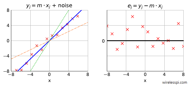
We start with plotting the error $e_j=y_j-m\cdot x_j$ on the right side of the above figure. Since the noise is Gaussian, the error samples $e_j$ assume both positive and negative values. Owing to this bipolarity, one criterion to find the best fit line is by minimizing the total absolute value squared of the error samples $\sum_j|e_j|^2$. This criterion is known as the Least Squares (LS) solution. Let us find out where it leads.
\[
\min \sum_j|e_j|^2 = \min \sum_j(y_j-m\cdot x_j)^2
\]

The above function forms a parabola which has a unique minimum. This function can be minimized by taking the first derivative and equating it to zero. This first derivative is given by
\[
\sum_j\frac{d}{dm}(y_j-m\cdot x_j)^2 = \sum_j 2(y_j-m\cdot x_j)(-x_j) = -2\sum_j x_j\cdot y_j +2m\sum_j x_j^2
\]

Equating it to zero to find the minimum gives
\begin{equation}\label{equation-line-slope}
-2\sum_j x_j\cdot y_j +2m\sum_j x_j^2 = 0 \qquad \Rightarrow \qquad \hat m = \frac{1}{\sum_jx_j^2}\sum_j x_j\cdot y_j
\end{equation}

This is known as the linear least squares solution because it minimizes the sum of squared absolute values of the error terms.

A Single User in a Cell

---

Turning to our problem, assume that there was only a single terminal in the cell that communicates with all the base station antennas (i.e., there is no interference) such that the channel gains from that user, say 1, to receive antenna $j$ is $h_{(1\rightarrow j)}$. With its modulation symbol denoted by $s_1$, the received signal $r_j$ at antenna $j$ can be written as
\[
r_j = s_1\cdot h_{(1\rightarrow j)} + \text{noise}, \qquad \qquad j = 1, 2, \cdots, N_B
\]

Comparing with the linear equation $y_j=m\cdot x_j$, we have the following corresponding parameters.
\[
\begin{aligned}
y_j \quad &\longrightarrow \quad r_j \\
m \quad &\longrightarrow \quad s_1 \\
x_j \quad &\longrightarrow \quad h_{(1\rightarrow j)} \\
\end{aligned}
\]

From Eq (\ref{equation-line-slope}), the solution $\hat s_1$ can be correspondingly written as
\[
\hat s_1 = \frac{1}{\sum_j |h_{(1\rightarrow j)}|^2}\sum_j h_{(1\rightarrow j)}^*\cdot r_j
\]

The two differences from the straight line solution, i.e., the absolute value squared and conjugate operation, appear because $h_{(1\rightarrow j)}$ is a complex number (the fading channel coefficient). Since $|h_{(1\rightarrow j)}|^2$ $=$ $h_{(1\rightarrow j)}^*\cdot h_{(1\rightarrow j)}$, we can write
\begin{equation}\label{equation-zf-single}
\hat s_1 = \left(\sum_j h_{(1\rightarrow j)}^*\cdot h_{(1\rightarrow j)}\right)^{-1}\sum_j h_{(1\rightarrow j)}^*\cdot r_j
\end{equation}

that is analogous to Eq (\ref{equation-optimal-weighting}). With this result in hand, it is straightforward to understand the Zero-Forcing algorithm for a multi-user scenario.

Multiple Users in a Cell

---

Now in reality, there is not a single user but multiple users in a cell which communicate with the base station at the same time and frequency thanks to favorable propagation scenario discussed in the last section. In such a case, hidden in the received data samples $r_j$ are not simply the modulation symbols $s_1$ from terminal 1 but also the modulation symbols $s_2$, $\cdots$, $s_K$ from all $K$ users. Therefore, the signal model $r_j$ $=$ $s_1\cdot h_{(1\rightarrow j)}$ becomes multi-dimensional as
\begin{equation}\label{equation-vector-model}
\mathbf{r} = \mathbf{H}\cdot \mathbf{s} + \textbf{noise}
\end{equation}

where $\mathbf{r}$ is a vector of received samples, $\mathbf{H}$ is a matrix whose entries $h_{(i\rightarrow j)}$ are channel gains from user $i$ to antenna $j$ and $\mathbf{s}$ is the vector of modulation symbols $s_1$, $s_2$, $\cdots$, $s_K$. Just like a single user where $\sum_j(y_j-m\cdot x_j)^2$ or $\sum_j(r_j-h_{(1\rightarrow j)}\cdot s_1)^2$ was minimized, the least squares solution now focuses on minimizing $||\mathbf{r}-\mathbf{H\cdot s}||^2$. Then, the solution can be straightforwardly written just like Eq (\ref{equation-zf-single}) or Eq (\ref{equation-optimal-weighting}) as
\begin{equation}\label{equation-zf-multiple}
\mathbf{\hat s} = \mathbf{\Big(H^*\:H\Big)}^{-1}~\mathbf{H^*\:r}
\end{equation}

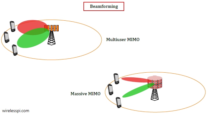
where the term before $\mathbf{r}$ is known as a pseudo-inverse of a matrix and $\mathbf{H^*}$ implies both a transpose and a conjugate operation on channel matrix $\mathbf{H}$. This is the expression you would have seen in most research papers and books on 5G physical layer algorithms. While this matrix result seems difficult to understand at first, I believe the derivation of a single user as in Eq (\ref{equation-zf-single}) helps in grasping the underlying basic idea. The enhancement of gains and nullifying the interference in the directions of other users with a massive number of antennas results in a system that is quite different from a simple multi-user system. This is illustrated in the figure below where the cost of additional antennas simplifies the system design in other aspects. Keep in mind that although physical beams are drawn in this figure, the idea stays the same for generalized beamforming scenario.

A few comments are in order here.

Why Zero-Forcing?

---

In the case of matched filter detector, we relied only on favorable propagation conditions to nullify the interference coming from $K-1$ users. We also mentioned that this only approximately holds true for a large number of antennas $N_B$. In the present instance, the algorithm is known as Zero-Forcing because the decoding vectors are structured in a way to nullify interference among the users, i.e., force zeros on the off-diagonal terms of the matrix. Let us find out how.

Plug in the value of the received samples $\mathbf{r}$ from Eq (\ref{equation-vector-model}) into the Zero-Forcing solution of Eq (\ref{equation-zf-multiple}), we get
\begin{align}
\mathbf{\hat s} &= \mathbf{\Big(H^*\:H\Big)}^{-1}~\mathbf{H^*}\:\Big(\mathbf{H}\cdot \mathbf{s} + \textbf{noise}\Big) \nonumber \\
&= ~~\mathbf{s} ~~+~~ \textbf{modified noise}\label{equation-noise-enhancement}
\end{align}

The operation $\mathbf{\Big(H^*\:H\Big)}^{-1}~\mathbf{H^*}\:\mathbf{H}$ equals $\mathbf{I}$ in the first term, where $\mathbf{I}$ is an identity matrix with ones along the main diagonal and zeros everywhere else. As a result, the signal part in the first term now contains only a vector with each user’s modulation symbol free of influence from the other symbols.

Noise Enhancement

---

One drawback of a Zero-Forcing solution is noise enhancement. Refer back to Eq (\ref{equation-noise-enhancement}) and focus on the effective noise part now. The problem with the multiplicative factor appearing with noise is that it is an inverse of a matrix, much like the expression $\big(\sum_j h_{(1\rightarrow j)}^*\cdot h_{(1\rightarrow j)}\big)^{-1}$ for a single user in Eq (\ref{equation-zf-single}) before. With these channel gains in the denominator, the effective noise can be enhanced at frequencies where channel gains assume low values. This enhanced noise then dominates the signal part and deteriorates the estimation performance.

Regularization Factor

---

From the above description, a balance between SNR enhancement and interference mitigation is required. One solution is to introduce an additional factor in Eq (\ref{equation-zf-multiple}) that limits the extent of inversion.
\[
\mathbf{\hat s} = \Big(\mathbf{H^*\:H}+\delta \mathbf{I}\Big)^{-1}~\mathbf{H^*\:r}
\]

where $\delta$ is a positive number known as a regularization factor that can be tuned to strike a tradeoff between the two techniques covered before.

• When $\delta\rightarrow 0$, the effect of channel dominates and this is clearly the Zero-Forcing solution of Eq (\ref{equation-zf-multiple}), i.e., $\mathbf{\hat s} = \Big(\mathbf{H^*\:H}\Big)^{-1}~\mathbf{H^*\:r}$.
• When $\delta\rightarrow\infty$, the identity matrix dominates the channel matrix and the inverse of $\mathbf{I}$ is close to identity $\mathbf{I}$ as well. This is clearly maximum ratio or matching filtering, i.e., $\mathbf{\hat s} = \mathbf{H^*\:r}$.

Regularized Zero-Forcing has proved to be a good candidate between complexity and tradeoff in implementation of massive MIMO in commercial networks.

Finally, on the downlink, a precoding matrix similar to Eq (\ref{equation-zf-multiple}) before data transmission enables the base station to beamform multiple data streams to all user terminals without causing any mutual interference among them. Due to a large number of base station antennas $N_B$, linear processing algorithms described above such as matched filtering and Zero-Forcing are nearly optimal in massive MIMO systems and computationally complex signal processing algorithms are not required.

It must be mentioned that there is a performance gap that exists between all the schemes. Optimal detection is better than Zero-Forcing that in turn performs better than maximum ratio or matched filtering. This makes sense because Zero-Forcing nullifies the interference layers beforehand that results in a significant improvement in SINR.