In a previous article, we described how multiples antennas can be viewed as sampling the signal in space domain in a direct analogy to sampling the signal in time domain. Filters in discrete-time domain are usually defined by numerical values in the time axis. Space allows three-dimensional freedom. A filter in discrete space can have its elements placed anywhere in the space. This sounds very complicated! But we will show it is not.
A Simple Time Domain Filter: 2-Tap FIR
The simplest discrete FIR filter has only two samples of unit magnitude. Assuming unit magnitude and zero phase for both samples. The response of this filter is in the blue curve. The response of this filter depends on the relative phase difference between the two samples. Usually, we keep the first sample fixed to the 0 phase. Changing the phase of the second sample modifies the filter’s frequency response. Why?
Let us think for a moment. If we multiply a two-sample rectangular window at index 0 and 1 to a discrete-time complex sinusoid of a particular frequency you get the two-tap filter under discussion. As we already know, multiplication in the discrete-time domain is convolution in the frequency domain. A complex sinusoid in the time domain is an impulse in the frequency domain. A rectangular window in the time domain is a sinc-function in the frequency domain. Now, the resulting frequency response is obvious!
It is important to always remember the Nyquest criteria: $T_s \le \tau/2$
The use of this filter as low-pass, band-pass, or high-pass is not very useful, as the pass-band covers almost all of the allowed frequency range. However, this filter is an excellent band-stop filter, as the stop-band is narrow, with a sharp transition. For example removing DC, 60Hz power-line noise, or any particular constant narrowband interference.

A Simple Spatial Filter: 2 Antenna Array
Similar to the FIR example, the most straightforward array is linear and made of only two antennas. We place the two elements on the y-axis and assume that the signal of interest is coming from the x-axis as a plane wave. In the time domain, we always take time index 0 as the reference to compute the delay, in the space domain we take the origin as the reference to the distance.

The distance between the two elements must fulfill Nyquist’s criteria for space-domain sampling. Since we are dealing with electromagnetic waves, they travel at the speed of light. The wavelength, $\lambda$ is the ratio of the speed of light $c$, to the frequency of the electromagnetic wave of interest, $ƒ$. The wavelength of frequency in space is equivalent to the time period of frequency in time, $\tau=1/f$. Therefore, in space, the distance d between the two antennas must be $\lambda/2$ or less to fulfill the Nyquist criteria of space-domain.
The direction of the source is measured as a change in angle in azimuth or elevation or both. The angle change in XY-axis is the azimuth angle, and YZ or XZ direction is the elevation angle. The angular change of the source in the space domain is equivalent to the frequency change of the signal in the time domain. A change in source angle also changes the relative distance between the two antennas. How?
A 2D project of the 3D diagram is shown to explain this phenomenon. The red dots are the actual position of the antennas. The blue dots are the projection of the antennas on the x-axis. Instead of changing the source angle, we choose to rotate the array.
Initially, the projection of the antennas falls on the same spot on the x-axis. Therefore, for the incoming plane wave, there is no delay between them. As we rotate the array we see an increase in the distance between the projected antennas. Rotating this array by $^\circ$ results in a distance equal to the actual antenna distance.

Computing the Steering Vector from the Projected Array
If we take the origin as the reference point. The delay is positive for positive values of the x-axis and negative the other way. The steering vector gives us the phase delay of the projected antennas for any angular displacement of the source from the array. This can be easily computed using trigonometry principles of right-angled triangles. In this example, initially, the array is parallel to the incident plane wave. The angle between them is zero. The distance between the projected antennas is also zero. Therefore, the phase experienced by the plane wave is also zero.
For any angular displacement, θ, the projection of the antenna is $(d/2)\sin \theta$. To convert it to phase delay we multiply it with $2\pi/\lambda$. Therefore, the steering vector is simply,
a(θ) = [ei2π(d/2)(sinθ)/λ e-i2π(d/2)(sinθ)/λ]T (1)
The Steering Vector and the Direction of the Signal Received by the Array
Suppose a plane wave signal, x(t), from an unknown source, is incident on our simple array. We will receive two signals, x1(t) and x2(t), from the two antennas of the array. How do we know from where the signal came? We will compute the phase of the two signals and compare them to the steering vector in (1) for different values of θ. When we find a match between the phases of the received signals and phases of the steering vector we can know from where the signal came.
In mathematical form we would do a dot product of the incoming signal vector with the steering vector to get a spatial spectrum:
p(θ) = [x1(t) x2(t)]*a(θ) (2)
This equation gives the magnitude spectrum in the angular domain. The spectrum peaks at the angle of arrival of the signal. The spatial spectrum angle of arrival at 0o, 45o, 68o, and 90o is shown below.

The Steering Vector and the Digital Beamforming
How can we use multiple antennas to form digital beams? Again the steering vector comes to the rescue. The values of the steering vector at a particular angle are the coefficient of the beamformer for that angle. Let us say we want our beam to be at 0o. We replace θ in (2) with 0. The spatial response of the beamformer is the same as the blue curve above. Again, this is not a very good beamformer in terms of directivity, just like our FIR filter. However, the purpose here was just to explain the basic concepts.
A Generalized Spatial Filter and its Steering Vector
By generalization we mean any array type with any number of antennas. A few array types are: rectangular, circular, cylindrical, conformal, and spherical. It is possible to derive a closed-form steering vector for each type. However, with computational power at hand, it is also possible to generalize a numerical method to find the values of the steering vector at any angle for any array type and with any number of antennas. The steps to get the values of the steering vector are:
- Define the antenna array in a 3D coordinate system by specifying the location of each element, [xi yi zi]T, as columns of a matrix M. The origin must be at the center of the array.
- Project the elements to the x-axis, this is simply done by only considering the first row of M which is, x.
- The steering vector at angle zero is ei2π(x)/λ.
- To compute the steering vector at azimuth angle θ and elevation angle φ, rotate the array M by θ using rotation matrix R(θ) and by φ using rotation matrix R(φ).
- Compute the steering vector in step 3 using x of the rotated array R(φ)R(θ)M.
Usually, we compute the steering vectors for angles in azimuth and elevation with 1o resolution and store them in a matrix, A. The spatial spectrum of the array for a particular direction of arrival signal can be computed easily using:
p(θ,φ) = aH(θ,φ)A … (3)
Example of Computing Beam-Pattern Using the Generalized Method for Computing Steering Vector
Now we take a more elaborative example of a 4×4 rectangular array. We use the method discussed above to compute the beam pattern. We see the pattern is symmetric over the positive and the negative x-axis. This is because we selected to an Omnidirectional element pattern. We dissect and remove the upper half to appreciate the beam pattern in azimuth. The effect of an element pattern on the overall beam pattern of the array is a topic for another day.

A Quick Review of the Rotation Matrix
A point in three-dimensional [xi yi zi]T space can be rotated in XY-plane, XZ-plane or YZ plane depending on the matrix R(ψ). The three types of rotation matrices are:

We use them individually or in combination as we did in the calculation of the steering matrix. Rotation matrices are a useful tool used in matrix decomposition and computer graphics.
Conclusion
In this article, we compare the Nyquist criteria of a simple 2-sample FIR filter with a simple 2-element linear array. Then we proceed to define the steering vector and its relationship to the array pattern and beamforming. Finally, we show a method to obtain the steering vectors for a generalized array.
This article is very poorly written compared to other articles in this forum.