We have described before how supervised learning can help us predict a continuous-valued output or organize the input into discrete categories, commonly known as regression and classification problems, respectively. In this article, we describe linear regression and leave the classification algorithms for a future post.
What is Linear Regression?
Suppose that you are a young investor living in a region with cold climate. One day an idea flashes in your mind that perhaps the shares in the regional stock market climb linearly with the temperature: the better the weather, the higher the prices.
- You already know what the temperature is going to be tomorrow.
- And you want to know the price of a particular stock for tomorrow.
Knowledge of linear regression is needed to solve this problem.

Given an input and output set, linear regression finds a straight line or some other curve between them such that new outputs can be predicted (on a continuous-scale) for given inputs. Assume that the input and output data sets are given by $x_i$ and $y_i$, respectively where $i=1,2,\cdots,N$ is the observation index. The purpose is to draw the inputs $x_i$ on the x-axis as independent variables and the outputs $y_i$ on the y-axis as dependent variables.
\[
y_i = m\cdot x_i + c \quad+\quad e_i
\]
where $m$ is the slope, $c$ is the y-intercept and $e_i$ is the error between each observation and the linear model. The figure below illustrates this process.

From there, the algorithm needs to fit a straight line through the data points that represents the best curve with respect to some criterion. For example, there are three candidate lines in the above figure. We can easily observe that the blue line is the best fit among these three choices but how our mind arrived at this conclusion is not clear. More importantly, how should a machine devise an algorithm that can pop out the best possible answer? For this purpose, we need a cost function as a starting point.
The Cost Function
A cost function is necessary as a performance indicator. The nature of the cost function then impacts the derivation of the optimal algorithm. The question is how to construct such a function.
For this purpose, see the image below of an alpine skiing scenario. Assume that the purpose of the athlete is to pass through a straight line between the poles, not around them. If there was only one set of poles, the strategy is to pass while keeping an equal distance from both right and left poles. For the realistic scenario, the skier should minimize the average distance between all such pairs.

AP Photo Giovanni Auletta
The line fitting scenario of the data set is not much different. We start with plotting the error $e_i=y_i-m\cdot x_i$ on the right side of the figure below for which we have assumed that the y-intercept $c$ is zero for clarity.

Since $e_i$ take both positive and negative values, we consider the squares of these error samples.
\[
|e_i|^2 = \big|y_i-m\cdot x_i – c\big|^2
\]
There are three lines with different slopes in the above figure. The cost function should be the minimum with one of them (the blue line) while higher than all the other slopes. This can be verified by plotting the error function against the line slopes on the x-axis as in the figure below. The minimum value is seen to be reached for $m=1$.

Owing to this bipolarity, one criterion to find the best fit line is by minimizing the average squared error $\frac{1}{N}\sum_i|e_i|^2$.
\[
\frac{1}{N} \sum_i |e_i|^2= \frac{1}{N}\sum _{i=1}^N \big|(y_i-m\cdot x_i – c\big|^2
\]
Having a cost function in hand, we can move towards the solution.
Non-Iterative Solution – Least Squares
If your data set is not large, you can find the solution by processing the available data in one go, i.e., a feedforward formula can be applied to get the answer. Let us explore how.
Finding the Slope
For simplicity, temporarily assume that the y-intercept $c$ is zero. Then, we have
\begin{equation}\label{equation-single-variable}
y_i = m\cdot x_i, \qquad i=1, 2, \cdots, N
\end{equation}
We can find the slope $m$ by minimizing the cost function as follows.
\[
\min \sum_i|e_i|^2 = \min \sum_i(y_i-m\cdot x_i)^2
\]
The above function forms a parabola which has a unique minimum. This function can be minimized by taking the first derivative and equating it to zero. This first derivative is given by
\[
\sum_i\frac{d}{dm}(y_i-m\cdot x_i)^2 = \sum_i 2(y_i-m\cdot x_i)(-x_i) = -2\sum_i x_i\cdot y_i +2m\sum_i x_i^2
\]
Equating it to zero to find the minimum gives
\begin{equation}\label{equation-line-slope}
-2\sum_i x_i\cdot y_i +2m\sum_i x_i^2 = 0 \qquad \Rightarrow \qquad \hat m = \frac{1}{\sum_ix_i^2}\sum_i x_i\cdot y_i
\end{equation}
This is known as the linear Least Squares (LS) solution because it minimizes the sum of squared absolute values of the error terms.
Finding the Slope and y-Intercept
When the y-intercept $c$ is not zero, it can be jointly estimated with the slope $m$ by following a similar methodology as above. To keep the discussion simple, we skip the mathematical steps and produce the exact solution below.
\[
\begin{aligned}
\hat m ~&=~ \frac{N\sum_{i=1}^{N}x_iy_i-\left(\sum_{i=1}^{N}x_i\right)\left(\sum_{i=1}^{N}y_i\right)}{N\sum_{i=1}^{N} x_i^2 – \left(\sum_{i=1}^{N}x_i\right)^2}\\
\hat c ~&=~ \frac{\left(\sum_{i=1}^{N} x_i^2\right)\left(\sum_{i=1}^{N}y_i\right)-\left(\sum_{i=1}^{N}x_i\right)\left(\sum_{i=1}^{N}x_iy_i\right)}{N\sum_{i=1}^{N} x_i^2 – \left(\sum_{i=1}^{N}x_i\right)^2}
\end{aligned}
\]
Here, you can simply plug the values in the above formula to get the best line fit for linear regression.
Multivariate or Multiple Linear Regression
Initially we said that as a young investor, you discovered a linear relation between the temperature and stock market performance. After a few days, you realize that the real world is not that simple. Many other variables impact the actual market such as the political situation, current events, overall health of the economy and even human emotions. Therefore, the output price is a function of several variables, not one.
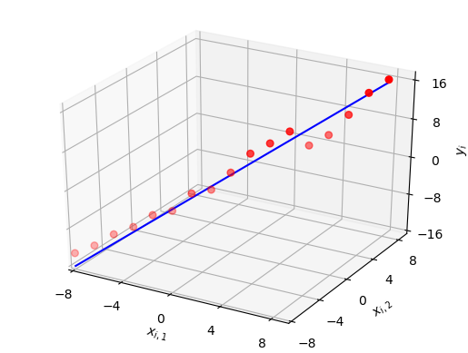
Assume that the relation is still linear, i.e. the output $y_i$ can be written as a function of three variables as
\[
y_i = a\cdot x_{i,1}+b\cdot x_{i,2}+c\cdot x_{i,3} + d
\]
This is still a linear plot but in multiple variables as shown in the figure below. This is why multivariate linear regression is also known as multiple linear regression.

These can now be written in a matrix form as
\begin{equation}\label{equation-multiple-variables}
\mathbf{y} = \mathbf{X}\cdot \mathbf{\theta}
\end{equation}
where $\mathbf{y}$ is the output vector, $\mathbf{X}$ is a matrix while $\mathbf{\theta}$ is a vector. Their entries are given by
\[
\mathbf{X} =
\begin{bmatrix}
x_{1,1} & x_{1,2} & x_{1,3} & 1\\
x_{2,1} & x_{2,2} & x_{2,3} & 1\\
\vdots & \vdots & \vdots
\end{bmatrix}, \qquad\qquad
\mathbf{\theta} =
\begin{bmatrix}
a \\
b \\
c \\
d
\end{bmatrix}
\]
Observe that Eq (\ref{equation-multiple-variables}) is quite similar to Eq (\ref{equation-single-variable}) where $\sum_i(y_i-m\cdot x_i)^2$ was minimized. Here, the least squares solution now focuses on minimizing $||\mathbf{y}-\mathbf{X\cdot \theta}||^2$. Therefore, the solution can easily be replicated from the scalar for of Eq (\ref{equation-line-slope}) as
\begin{equation}\label{equation-multiple-solution}
\mathbf{\hat \theta} = \mathbf{\Big(X^T\:X\Big)}^{-1}~\mathbf{X^T\:y}
\end{equation}
where the superscript $T$ stands for transpose. Keep in mind that when a complex data set is involved, both transpose and conjugate operation need to be implemented.
Iterative Solution – Gradient Descent
What happens when your data set is large and you do not have enough computing power to invert large matrices in Eq (\ref{equation-multiple-solution})? In this more realistic scenario, an iterative solution is better suited to the job where the algorithm starts from an initial state and converges towards the final estimates of unknown variables in a step-by-step manner. This brings us to the gradient descent technique for a single variable.
Updating the Slope
In a previous article on LMS equalization, we saw how a gradient is just a mere generalization of the derivative (slope of the tangent to a curve) for a multi-variable function through the example of a roller coaster.
Recall the quadratic cost function discussed before in this article and observe how it is similar to that roller coaster for a single variable, the slope $m$ of the line. This is shown in the left figure below along with the directions of gradient and its opposite.

On the same note, the right figure draws the same relationship as a quadratic surface of two variables where a unique minimum point can be identified. We cannot graphically draw the same relationship for a higher number of variables.
We can start at any point on this error curve curve and take a small step in a direction where the decrease in the squared error is the fastest. The fastest reduction in error happens when our direction of update is opposite to the gradient of $|e_i|^2$ with respect to the slope.
\[
m = m + \text{a small step opposite to the gradient of}~\sum_i|e_i|^2
\]
The gradient is a mere generalization of the derivative and a minus sign is brought for moving in its opposite direction.
\[
m = m – \alpha \cdot \frac{\partial}{\partial m}\sum_i|e_i|^2
\]
where $\alpha$ is the step size in the algorithm. The minus sign plays the following role as shown in the figure below.

- For positive slope (the right of the optimal point), the derivative is positive and minus sign pulls the updated value $m$ back towards the left.
- For negative slope (the left of the optimal point), the derivative is negative and minus sign makes it positive thus pushing the updated value $m$ forward towards the right.
Step Size
The significance of step size $\alpha$ is as follows.
- A large value of $\alpha$ generates a response that converges faster than that for a smaller value of $\alpha$. This makes sense because a large $\alpha$ necessitates a large update in the current value.
- So why not choose $\alpha$ as large as possible? A larger $\alpha$ results in a greater excess error and can even result in divergence due to large updates.
In light of the above, the value of $\alpha$, known as learning rate, is chosen to strike a balance between rapid convergence and excessive overshooting.
Multivariate or Multiple Linear Regression
In this case of two or more variables, the error curve transforms into an error surface as shown before for two variables. We again adopt a gradient descent approach to derive the update equations as follows.
\[
\begin{aligned}
m &= m – \alpha \cdot \frac{\partial}{\partial m}\sum_i|e_i|^2 \\
c &= c – \alpha \cdot \frac{\partial}{\partial c}\sum_i|e_i|^2
\end{aligned}
\]
The derivative for two variables can be derived as follows. For the slope $m$, we have
\[
\begin{aligned}
\frac{\partial}{\partial m}|e_i|^2 &= \frac{\partial}{\partial m} \left(y_i-m\cdot x_i – c\right)^2 \\
&= \left(y_i-m\cdot x_i – c\right) (-x_i)
\end{aligned}
\]
where we have ignored the irrelevant constants $2$ and $N$ that can be absorbed in $\alpha$. Similarly, for the y-intercept $c$, we get
\[
\begin{aligned}
\frac{\partial}{\partial c}|e_i|^2 &= \frac{\partial}{\partial c} \left(y_i-m\cdot x_i – c\right)^2 \\
&= -\left(y_i-m\cdot x_i – c\right)
\end{aligned}
\]
where the irrelevant constants $2$ and $N$ have been absorbed in $\alpha$ again. From the above expressions, the algorithm can now be written as
\[
\begin{aligned}
\tilde m &= m + \alpha \sum_i\left(y_i- m\cdot x_i – c\right) (x_i) \\
\tilde c &= c + \alpha \sum_i\left(y_i- m\cdot x_i – c\right) \\
m &= \tilde m \\
c &= \tilde c
\end{aligned}
\]
where $\alpha$ is the learning rate, $x_i$ and $y_i$ are the values in the data set, while $m$ and $c$ are the variables to be estimated for the line fit. The notations $\tilde m$ and $\tilde c$ are included because previous value of $m$ should be used for updating $c$ (in reality, the notations $\hat m$ and $\hat c$ should be used that is avoided here to keep the equations look simpler).
If we include the entire training set in every step, the above algorithm is called batch gradient descent. Otherwise, if the summation is removed and the estimates are updated with each new observation, this becomes similar to a least mean squares approach.
Finally, this can be generalized to multiple variables in a straightforward manner.
\[
\theta_j = \theta_j – \alpha \cdot \frac{\partial}{\partial \theta_j}\sum_i|e_i|^2
\]
Prediction
Having the coefficients estimates in hand, we can now construct the model that is best supposed to generate the target system output.
\[
y_i = \hat m \cdot x_i + \hat c
\]
Clearly, when the input $x_i$ is known, it can be plugged in the above equation to predict the output. In our original example of simple linear regression analysis, the investor can plug in tomorrow’s temperature $x_i$ to find the stock price $y_i$ beforehand.
For example, if $\hat m = 1.2$ and $\hat c = -2.3$, we have
\[
y_i = 1.2x_i -2.3
\]
If tomorrow’s temperature is forecast as $31^\circ$ C, then the price is predicted as \$34.9.
Concluding Remarks
A few remarks are in order now.
- Data Preparation
There are several data preparation steps that are recommended to perform before regression analysis. For example, correlation between different pairs of input variables needs to be found and the one with the highest correlation with another input variable can be removed. Moreover, input variable normalization is utilized by most machine learning algorithms. This is because different inputs can have a wide range of variances that can impact the coefficients estimation. If they are adjusted to zero mean and scaled by their own variances, contribution from a single input variable cannot drown out those from the rest.
- Gaussian Distribution
- Performance metrics
- Total Least Squares
The squared differences are shown as vertical lines in the figure below. Keep in mind that this least squares solution targets the squared vertical lengths only and hence implicitly assumes that inputs $x_i$ are perfect. In the real world, many input observations $x_i$ are also subject to noise and errors and the optimal solution is to minimize the sum of squared projections (perpendicular lines or shortest distances) from the red dots onto the blue line. This is solved through a method known as Total Least Squares.
- Regularization
Regularization methods are used to simplify the least squares solution when there is correlation between the input data. That will be the covered in a future article.
- Classification
There are other algorithms one can employ for classification problems such as logistic regression and k-Nearest Neighbors (k-NN).
- Finally, you can the read articles on Artificial Intelligence (AI) here.
Least Squares is the optimal solution if errors in the model follow a normal distribution. For other error distributions, better estimation techniques are available. Nevertheless, this method is still the best linear unbiased estimator among all the possible techniques.
One of the most commonly used metric as a performance benchmark is R-squared. This metric evaluates the scatter of the data points around the regression line generated from our estimates.
\[
R^2 = 1 – \frac{\sum_i |e_i|^2}{\sum_i (y_i-\bar y)^2}
\]
where $\bar y$ is the sample mean. A value closer to 1 indicates a model that is a good fit. Other performance metrics such as mean square error (MSE) or root mean square error (RMSE) are also common.