A hundred thousand years ago, our ancestors used to roam in the savannas and jungles. It was absolutely necessary for them to judge (or classify) everything they encounter: a movement in the bushes could be due to a harmless rabbit or a dangerous tiger, a fruit on a plant could be nutritious or poisonous, and so on. Then came the wizards who invented language and then people developed agriculture, writing and industry. The advancement in civilization and the quest for scientific knowledge revealed the benefits of a wide spectrum and viewing shades of gray instead of of simple black and white realities.
The interesting thing is that decision making still requires classification. We simply cannot have an open mind or 50-50 opinions for important decisions. This task, however, is being gradually taken over by the machines.
- One of the reasons for the rise of Gmail was excellent spam filters by Google, even though other competitors had a head start of several years. Email would have been a thing of the past if the filters were not separating the spam from intended emails.
- Using a range of indicators, an algorithm needs to recommend a decision whether a particular stock is worthy of investment or not.
- During the Musk-Twitter battle, Elon Musk accused Twitter of of fraud for hiding the real number of fake accounts. How can a machine differentiate a legitimate account from a fake one?

The Generator of Reality
A binary classification of a problem into clear black and white categories implies assigning them the states 0 and 1. The question is: how can we do that based on a set of data that is continuous in nature and can range from very small to very large numbers?
In the article on linear regression, we have already seen the curve fitting between an input set $x_i$ and output set $y_i$. that approximates the underlying relationship between them. Here, we introduce an intermediate variable $z$, the reason for which soon becomes clear. For a linear curve with one variable,
\begin{equation}\label{equation-linear-regression}
z = \theta_0+\theta_1\cdot x
\end{equation}
We then treat this curve fit through $\theta_0$ and $\theta_1$ as a true generator of reality, i.e., new predictions about the output $z$ can be made for a different input $x$.
Our current problem is that of binary classification. The input is a set of data with information about different features and we have to assign them to a class $y=0$ or $y=1$, given the reality-generating curve. In this setup, we can take help from the same methodology as linear regression but in a different way. Let us find out how.
From a Continuum to a Discrete Set
Here is what we can do.
- We have the data set $x_i$ and $z_i$. We have also discovered the underlying relation that generates them, i.e., the curve fitting parameters $\theta_0$ and $\theta_1$.
- This output can be mapped to another function that limits the original range between 0 and 1, thus satisfying our binary classification criterion. One such function is known as the logistic function, also called a sigmoid function. For the variable $z$, it is given by
\[
LF(z) = \frac{1}{1+e^{-z}}
\]As shown in the plot below, the shape of this curve approaches 0 for negative values and 1 for positive values.
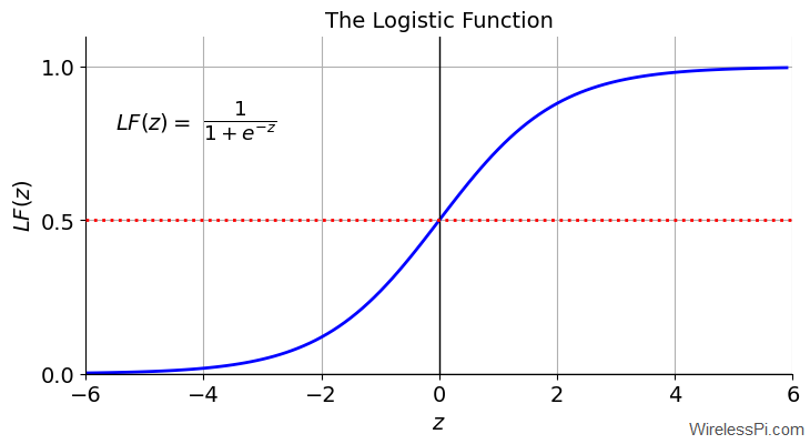
Plugging in the expression for $z$ from Eq (\ref{equation-linear-regression}),
\[
LF(z) = \frac{1}{1+e^{-(\theta_0 + \theta_1 x)}}
\]From the red dotted line serving as a threshold in the above figure, we can now classify the output $y$ by the following rule.
\[
\begin{aligned}
LF(z) \ge 0.5 &\qquad\longrightarrow \qquad y = 1 \\
\\
LF(z) < 0.5 &\qquad\longrightarrow\qquad y = 0 \end{aligned} \]In summary, the algorithm predicts $y=1$ if $LF(z)\ge 0.5$ and $y=0$ otherwise. In words, it assigns class 1 to the data points for which the logistic function output is greater than $0.5$ and class 0 to the remaining data set.
Decision Boundaries
In general, the data points are plotted such that the outputs are on the y-axis and the inputs are on the x-axis. The question is how to draw a decision boundary without the mapping in the logistic function. Here is what we do.
Observe from the logistic function figure that the condition $LF(z)=0.5$ is the same as $z=0$. This can be utilized to mark the decision boundary. Recalling the value of $z$ from Eq (\ref{equation-linear-regression}),
\[
z = \theta_0+\theta_1\cdot x = 0
\]This implies that
\[
x = -\frac{\theta_0}{\theta_1}
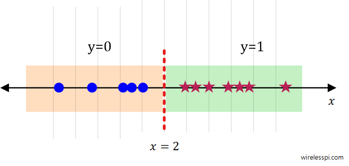
\]For an example of $\theta_0=4$ and $\theta_1=-2$ that are obtained from a trained model, we have the decision boundary as
\[
x = 2
\]As drawn in the figure below, the values to the right of this line are classified as $y=1$ and the values to the left are assigned as $y=0$.
Next, we describe how to go from a single variable logistic regression to multivariate logistic regression.
Multivariate Logistic Regression
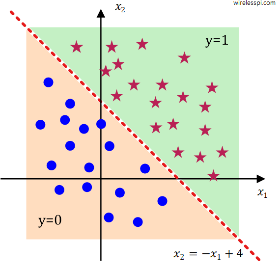
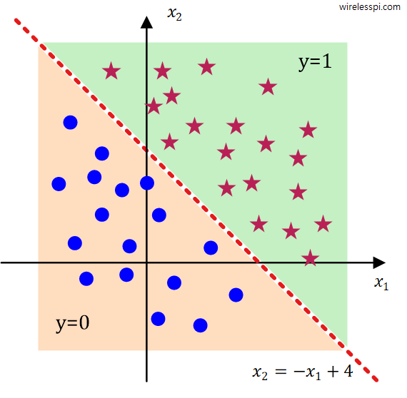
It is also possible to extend this single variable idea into a multiple variable one. Assume now that there are two independent variables $x_1$ and $x_2$ and the linear curve is given as
\[
z = \theta_0 + \theta_1\cdot x_1 + \theta_2\cdot x_2
\]According to the description above, the decision boundary lies at $z=0$. In other words,
\[
\theta_0 + \theta_1\cdot x_1 + \theta_2\cdot x_2 = 0
\]For example values of $\theta_0=4$, $\theta_1=-1$ and $\theta_2=-1$, this implies that
\[
4 -x_1 -x_2 = 0, \qquad \qquad x_2 = -x_1 +4
\]As drawn in the figure below, the values above this line are classified as $y=1$ and the values below are assigned as $y=0$.
In a similar manner, this decision boundary can be non-linear for a non-linear curve.
Conclusion
In conclusion, we proceed as follows.
- Given the training data $(x_i, z_i)$, we come up with an underlying relation $z$ in terms of $\theta_i$ that generated them.
- In linear regression, we predict a value for an unknown output $y$ from a continuous range according to a new input $x$.
- In logistic regression, we assign a value for an unknown output $y$ from a discrete set according to a new input $x$.
Another algorithm one can employ for classification problems is the k-Nearest Neighbors (k-NN).