FIR vs IIR Filters – A Practical Comparison

When it comes to practical applications, digital filter design is one of the most important topics in digital signal processing. Today we discuss a critical question encountered in filter design: how to compare the Finite Impulse Response (FIR) and Infinite Impulse Response (IIR) filters. Since there is no clear winner, answering this question enables a designer to choose the right solution for their product.

A brief comparison of FIR vs IIR filters is now explained below.

Computational Complexity

---

It is well known that most practical signals are simply sums of sinusoids. This implies that signals with sharp transition in time domain are made up of a large number of constituent sinusoids, including those with higher frequencies. This is because rapid transitions in the original signal cannot be constructed from slowly varying smooth sinusoids. In other words, a signal narrow in time domain is wide in frequency domain.

Considering its dual, a spectrum with a sharp transition band necessitates a large duration in time domain. Therefore, a larger number of coefficients are needed for a given transition bandwidth and stopband attenuation in the FIR filters. This higher filter order results in higher computational complexity which becomes critical for some applications where sufficient processing power and memory storage are not available. An approximation (published by none other than fred harris) for determining the number of taps $N$ linking the normalized transition bandwidth (i.e., $\Delta f/F_s$) and stopband sidelobe levels is given by
\[
N = \frac{\text{Attenuation (dB)}}{22}\frac{F_s}{\Delta f}
\]

The question is, why do IIR filters require a far lesser number of coefficients as compared to FIR filters? For a given transition bandwidth and stopband attenuation, IIR filters can provide the same performance with less complexity because they employ their previous outputs as well, the outputs that carry within themselves a summarized effect of even more input samples from the past. FIR filters have no such benefit of feedback from the previous outputs.

Stability and Finite Precision Arithmetic

---

IIR filters are susceptible to numerical stability issues and coefficient quantization errors along the implementation stages. While their magnitude and phase responses can be verified before their deployment, the hidden dangers lie in the quantization noise.

There is a significant difference between FIR and IIR filters when it comes to the noise transfer function. This noise transfer function is similar to the signal transfer function from input to output ($Y(z)/X(z)$, known as the frequency response), but within the internal nodes where rounding or truncation is done. If implemented properly in fixed point, the FIR filters have the quantization noise variance simply scaled by the order $N$ that can be easily kept below the final quantization at the output.

In the IIR filters on the other hand, the quantization noise will scale in a similar manner but will go through the recursive portion of the filter. If the poles are located near the unit circle, the noise will be significantly amplified. Intuitively, the past quantization noise is repeatedly fed back into the filter, leading to a point where it can build to very large levels.

To overcome this problem, not only the actual quantization noise variance needs to be evaluated but it should also be minimized using suitable architecture due to its sensitivity to the order of operations. Noise shaping by feeding back the fractional errors after truncation can also be employed.

In summary, even if the IIR filter looks like a more suitable solution, this might not necessarily be the case once implemented in fixed point.

Overflow Oscillations

---

Thanks to Dan Boschen for putting it that well for me. IIR filters if not properly implemented with saturation detection on the output (to prevent overflow) can go into disastrous overflow oscillations which once started continue even if the input is brought to zero. If overflow is not prevented on a per sample basis, the fixed-point operations will insert a gross error in the output due to the wrap-around that takes place with 2’s complement arithmetic, which then gets fed back into the filter and the filter can then go into an oscillation that is some cases can be peak-to-peak of the output range.

Note that this is specific to the output stage in any IIR section, not necessarily an internal node. For example, consider the Direct Form I realization shown in the figure below, where there is functionally a single internal accumulator.

We may do the internal summations in such a way that an overflow temporarily occurs while all the nodes are getting added up (for a given input sample). It is interesting to note that this would be totally fine, as long as in the end (for that given sample), the output is within range with no overflow. It is this output that we may truncate down to the output precision and which gets fed back into the accumulator and it is that point specifically where we must not overflow when that sample gets fed back.

Why can we overflow internally in this case? Because of the way modulo math works, we can add an infinite amount of numbers and overflow an infinite amount of times as long as we eventually in the adding and subtracting come back to the primary range for our final result, all the math is still intact! As an example, consider the following expression in infinite precision arithmetic.
\[
5-7+4-1 = 1
\]

If this is implemented with 3-bit precision (which ranges from -4 to +3) as shown in the figure below, we would get
\[
(-3) + (1) + (-4) + (-1) = -7 = (1)
\]

where the parentheses () are used to represent the results after overflow. The results of both of the above equations are the same.

Limit Cycles

---

This is also called a "Zero Input Limit Cycle". Due to the feedback of quantized values in the IIR structure, we can end up with a small truncation error that gets fed back alternatively positively and negatively with no input. This is typically a very small level limited to the LSB (Least Significant Bit) or a few LSBs so the typical solution is to just ensure you add enough bits to the output precision so that this is below any noise floor you may have. In contrast, FIR filters will go to true zero after their memory length when the input goes to zero which is a significant advantage of FIR structures.

Linear Phase

---

For FIR filters, a linear phase can be simply achieved through symmetric or anti-symmetric coefficients that result in a constant group delay. The group delay is defined as
\[
\text{Group delay} = -\frac{d\theta(\omega)}{d\omega}
\]

where $\theta(\omega)$ is the phase response of the filter. The significance of the group delay is that it is a measure of average time delay taken by the input signal to pass through the filter. For a communications signal, it is desirable for the group delay to be a constant (i.e., a linear phase response) so that all frequency components are delayed by the same amount, thus preserving the signal shape and preventing any distortion. This is due to the reason that a delay appears as a linear frequency term in the phase term of the spectrum.
\[
x(t-\tau) \quad \rightarrow \quad e^{-j\omega \tau}X(\omega)
\]

where $X(\omega)$ is the Fourier Transform of $x(t)$ and the derivative of the phase term with respect to frequency can be seen to be the constant delay $\tau$. For a linear phase length-$N$ FIR filter, where $N$ is odd, the group delay is given by
\[
\text{Group delay} = \tau = \frac{N-1}{2}~\text{samples}
\]

which comes from the Discrete Fourier Transform (DFT) of the filter impulse response with symmetric or anti-symmetric coefficients.

For an IIR filter, it is impossible have an exact linear phase. Therefore, an all-pass filter (constant magnitude) with an inverse phase response can be cascaded with the IIR filter to achieve this objective.

A Filtering Example

---

Let us consider the problem of filtering a communication signal with the parameters shown in the figure below.

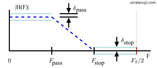
In this case, of particular importance is the fact that the sample rate $F_s=192$ kHz is much higher than the transition bandwidth of $13$ kHz.
\begin{align*}
&\text{Sample rate}, \quad F_s = 192\: \text{kHz} \\
&\text{Passband edge} \quad F_{\text{pass}} = 12\: \text{kHz} \\
&\text{Stopband edge} \quad F_{\text{stop}} = 25\: \text{kHz} \\
&\text{Passband ripple} \quad \delta_{\text{pass,dB}} = 0.1\: \text{dB} \\
&\text{Stopband ripple} \quad \delta_{\text{stop,dB}} = -75\: \text{dB}
\end{align*}

As evident from the above figure, the maximum amplitude in the passband of frequency domain is $1+\delta_{\text{pass}}$. These dB units can be converted into linear terms as
\begin{align*}
20 \log_{10} \big(1+\delta_{\text{pass}}\big) &= \delta_{\text{pass,dB}} \\
1+\delta_{\text{pass}} &= 10^{\delta_{\text{pass,dB}}/20} \\
\delta_{\text{pass}} &= 0.012
\end{align*}

Such a low value is chosen to preserve the desired signal with negligible Inter-Symbol Interference (ISI). As far as the stopband is concerned, we have
\begin{align*}
20 \log_{10} \delta_{\text{stop}} &= \delta_{\text{stop,dB}} \\
\delta_{\text{stop}} &= 10^{-75/20} = 0.00018
\end{align*}

If we design a run-of-the-mill FIR filter with Parks-McClellan algorithm for these specifications, it will have $N=53$ coefficients. Therefore, its workload is as follows.

Operation	Count
Multiplications	53
Additions	52
Multiplications/input sample	53
Additions/input sample	52
Group delay	135 $\mu$s

How did we compute the group delay as $135~\mu$s? For $N=53$, we have
\[
\text{Group delay} = \frac{53-1}{2} = 26~\text{samples}\approx 135~\mu\text{s}
\]

because at $F_s=192$ kHz, each sample appears after a duration of $1/F_s=5.2~\mu$s and $26$ samples span a duration of $26\times 5.2$ $\mu$s.

For each input sample, 53 multiplications and 52 additions is quite some work. Therefore, let us explore some other simpler options. Keep in mind that a low group delay is one of the main design criteria.

IIR Filter + All-Pass Equalizer

---

Among different kinds of IIR filters, a maximally flat group delay is exhibited by a Bessel filter. However, during the transformation to a digital equivalent (e.g., bilinear), this flatness is not reflected due to frequency warping. Moreover, direct design of digital IIR filters can have a stability concern. Therefore, we focus on an elliptic filter that has the lowest order for any given stopband attenuation.

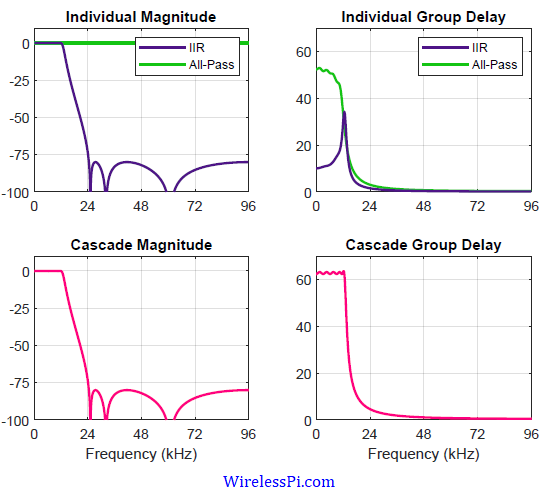
Using the Matlab filter design routine, an IIR filter of order $N_1=6$ seems to achieve the desired passband and stopband ripple. Within the passband, this filter has a variable group delay, reaching a peak of 35 samples for some frequencies near the passband edge. This creates distortion in the desired signal and must be equalized with an all-pass filter. An all-pass filter with $N_2=8$ seems to do the job.

The individual and cascade frequency responses of the IIR + all-pass combination, in addition to their respective group delays, are plotted in the figure below.

The top right figure demonstrates how a rising group delay of the IIR filter is compensated by a falling group delay of the all-pass equalizer. It is also evident from the bottom right figure that the group delay of the cascade becomes approximately 63 samples, or
\[
\text{Group delay} = 63/192,000 \approx 328~\mu\text{s}
\]

As far as the computational complexity is concerned, recall that higher-order IIR filter are mostly implemented through a cascade of 2nd-order IIR filters (quadratic polynomials in the numerator and denominator) which are known as biquad filters.
\[
\frac{Y(z)}{X(z)} = \frac{b_0+b_1z^{-1}+b_2z^{-2}}{1+a_1z^{-1}+a_2z^{-2}}
\]

where we have ignored the scaling factor. The expression for $y[n]$ can be found through inverse z-Transform.
\[
y[n] = b_0x[n]+b_1x[n-1]+b_2x[n-2] – a_1y[n-1]-a_2y[n-2]
\]

The reason is that these biquad sections are less prone to numerical stability issues, coefficient quantization errors and potential bit growth problems which makes them suitable for fixed-point implementations. A single biquad section (in Direct Form I structure) is drawn in the figure shown before during the discussion on overflow oscillations.

It is clear that implementation of each such a biquad section requires 5 multiplications and 4 additions. Therefore, for an IIR filter of order 6 (i.e., 3 biquads) and all-pass filter of order 8 (i.e., 4 biquads), we have approximately 35 multiplications and 28 additions for each input sample. This is summarized in the table below.

Operation	Count
Multiplications	35
Additions	28
Multiplications/input sample	35
Additions/input sample	28
Group delay	328 $\mu$s

Next, we consider the option of a halfband filter in cascade with an FIR filter and see how multirate techniques result in an efficient solution.

Halfband + FIR filter

---

In the original FIR filter, the transition bandwidth, given by $25-12$ $=$ $13$ kHz, is quite narrow as compared to the sample rate 192 kHz that necessitates an FIR filter with dozens of taps. If this sample rate is brought down, then the (normalized) transition bandwidth becomes large enough to allow FIR filtering with fewer coefficients.

• For this purpose, let us bring the sample of 192 kHz down to 96 kHz through a halfband filter whose specifications are as follows.
  \begin{align*}
  &\text{Sample rate}, \quad F_s = 192\: \text{kHz} \\
  &\text{Decimation factor} \quad D = 2 \\
  &\text{Transition bandwidth} \quad T_{\text{BW}} = 72\: \text{kHz} \\
  \end{align*}

  The transition bandwidth is $72$ KHz because the signal bandwidth is $12$ kHz and the first replica is going to appear at the new sample rate of $96$ kHz. This implies that we do not have any filtering concern for the region between $12$ and $84$ kHz that turns out to be $72$ kHz. The spectrum within this region is going to be filtered by the FIR filter coming next.

  This halfband filter is designed by just $N_1=7$ taps, out of which 2 are zeros at indices $n=\pm 2$ . Consequently, there are 5 multiplications and 4 additions, or 2.5 multiplications and 2 additions per input sample, respectively. The group delay is given by
  \[
  \text{Group delay} = \frac{7-1}{2}=3~\text{samples}\approx 15.6~\mu\text{s}
  \]

  The magnitude response and group delay of both the halfband filter and the FIR filter discussed next are plotted in the figure below.

  

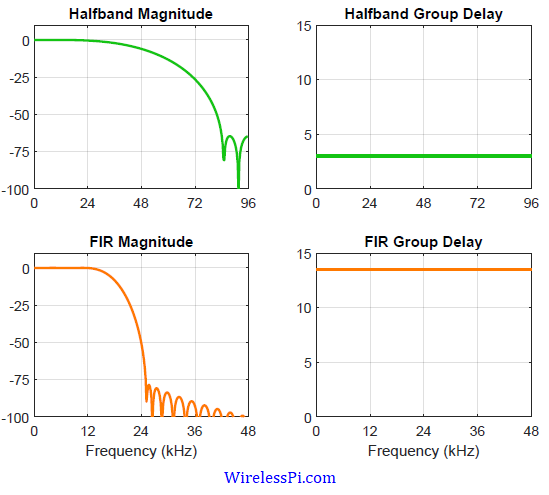
• An FIR filter now has an easier job with a normalized transition bandwidth of $13/96\approx 0.14$. Using the filter design routine again, an FIR filter with $N_2=28$ taps is enough for this task. The number of multiplications and additions are then 28 and 27 per input sample, respectively, at the low rate. At the original rate, this equals 14 multiplications and 13.5 additions per input sample. The group delay is computed to be 13.5 samples which is $140~\mu$s at $F_s=96$ kHz.

The total workload is computed by adding the results from the halfband and FIR filter as follows.

Operation	Count
Multiplications	5+28=33
Additions	4+27=31
Multiplications/input sample	2.5+14=16.5
Additions/input sample	2+13.5=15.5
Group delay	15.6+140 =155.6 $\mu$s

Finally, from an efficiency perspective, it is better for the modem to run the signal processing algorithms at the lower rate. However, if bringing the signal back to 192 kHz is necessary, then the output signal from the above cascade can be interpolated by another (interpolating) halfband filter. The total workload will increase by 2.5 multiplications and 2 additions along with an excess group delay of 15.6 $\mu$s.

Concluding Remarks

---

An IIR filter is generally chosen if the linear phase is not important and memory requirements are strict. This is why they are deployed in a wide range of products implementing audio and biomedical signal processing algorithms.

FIR filters are overwhelming used in applications such as digital communication systems where preserving the signal shape is of utmost importance (hence a linear phase) and required memory and computational power are available.

Finally, even in situations where the sample rate is much higher than the transition bandwidth and an IIR solution seems better, multi-rate techniques provide a tradeoff between number of multiplications, clock rate and memory. In particular, a decimating filter is more efficient in terms of multipliers and clock rate at the expense of more memory. This stays true even if another interpolating filter is also required for going back to the original sample rate. Moreover, this is a perfectly linear phase solution that can be easily extended to highpass and bandpass applications.

From here, you can also learn about the Goertzel algorithm that implements both IIR and FIR sections in a single filter.