June 18, 2020

---

---

---

On a cold morning in August 2015, I narrowly missed a train to my office in Melbourne city. With nothing else to do in the next 20 minutes, my mind wandered towards an intuitive view of complex numbers, something that has puzzled me since long. In particular, I wanted to seek answers to the following questions.

(a) What is the role of the number $\sqrt{-1}$ in mathematics? What sets it apart from other impossible numbers, e.g., a number $k$ such that $|k|=-1$? (The origins of this question might lie in how I cut apple slices for my kids as compared to my wife, see the figure below. I guess that many other dads also take this path of least resistance in trivial matters.)

(b) Why is $\sqrt{-1}$ a rotation by $90^\circ$ in a 2D plane? A square root and a rotation do not seem to be related at all.
(c) Why is the expression $e^{i \theta}$ a rotation of 1 by $\theta$ radians on a unit circle? Is it possible to make sense out of a number like $2.71828^{\sqrt{-1}\cdot\theta}$?

The ideas I wrote were forgotten in my notebook but this puzzle was reignited in my mind a few weeks ago. By the time you finish this guide, you will have answers to all three questions above and your way of looking at complex numbers will probably change forever. It should be kept in mind, however, that complex numbers can still be utilized without using any of these constants. In my books Wireless Communications from the Ground Up — An SDR Perspective or 5G Physical Layer, for example, I have not used $e$, $i$ or $j$ and still covered in depth how Digital Signal Processing (DSP) is applied to the design of wireless communication systems — a field known as Software Defined Radio (SDR).

Table of Contents

---

1. Gauss was Wrong, Descartes and Euler were Right

---

The history of imaginary numbers can be summarized in three quotes from three greatest mathematicians of their respective centuries.

Figure 1: Descartes, Euler and Gauss

• The square roots of negative numbers were called sophisticated or subtle before the publication of La Geometrie by the French mathematician Rene Descartes in 1637. He named them imaginary due to the impossibility of having a geometric construction for them and ignored possibly complex solutions to his equations. However, at the very last line of La Geometrie, he said: "I hope that posterity will judge me kindly, not only as to things which I have explained, but also as to those which I have intentionally omitted so as to leave to others the pleasure of discovery."
• Then, we have Leonhard Euler writing in his Algebra of 1770: "All such expressions as $\sqrt{-1}$, $\sqrt{-2}$, etc., are consequently impossible or imaginary numbers, since they represent roots of negative quantities; and of such numbers we may truly assert that they are neither nothing, nor greater than nothing, nor less than nothing, which necessarily constitutes them imaginary or impossible."
• Finally, Carl Friedrich Gauss wrote in 1831: "If this subject has hitherto been considered from the wrong viewpoint and thus enveloped in mystery and surrounded by darkness, it is largely an unsuitable terminology which should be blamed. Had $+1$, $-1$ and $\sqrt{-1}$ instead of being called positive, negative and imaginary (or worse still, impossible) unity, been given the names, say, of direct, inverse and lateral unity, there would hardly have been any scope for such obscurity."

Today it is customary to follow the perspective mentioned by Gauss to view and understand the complex numbers. However, I must say that the viewpoints of Descartes and Euler described above were correct and it was Gauss who underestimated the complexity of complex numbers, as explained in detail in the coming sections.

2. A Little Background

---

My initial resource to understand a concept is to refer to the textbooks written by the experts. The first textbook I read for this purpose contained the following definition.

"A complex number is an ordered pair $(a,b)$ of real numbers. “Ordered” means that $(a,b)$ and $(b,a)$ are regarded as distinct if $a\neq b$."

It was followed by the addition and multiplication rules as well as the definition of $i$ and its use as $\sqrt{-1}$. This reminded me of a quote by Georges Clemenceau: "War is too serious a matter to entrust to military men." I humbly want to modify it as "Mathematics is too interesting a subject to entrust to mathematicians." This is due to what psychologists call the curse of knowledge. Mathematicians, like all other professionals, have their own elevated boxes for thinking which are often unsuitable for teaching outsiders with little knowledge of mathematics. Probably a better strategy for maths teachers is to strike a balance between depth and breadth, e.g., by learning often underrated arts subjects.

My next resource to learn something is great online tutorials because top-ranked Google pages have almost never disappointed me in this regard. However, most of the popular resources on complex numbers introduce imaginary numbers with the statement

"Let’s assume some number $i$ exists where $i^2=-1$."

Or in a slightly changed version, $i$ is a root to the equation $x^2+1=0$. Next, they follow a path similar to what I first learned in high school. We were told that as long as we keep plugging in $\sqrt{-1}$ for $i$ and remember some basic rules, all the maths just works out (which turned out to be true). According to them, just like negative numbers indicate a place to the left of the origin, $\sqrt{-1}$ indicates a place above the number line. This new dimension — perpendicular to the original real line — was simply hidden from the narrow view of ordinary people. Thus declaring the imaginary numbers as original as natural, rational and irrational numbers, many such tutorials blame an intellectual deficiency on the reader’s part for the confusion regarding the absurd expression of $\sqrt{-1}$.

While I feel grateful to them for the wonderful job of making these difficult concepts easier, this is a perspective I find (unintentionally) disrespectful to the reader. If almost every learner finds imaginary numbers unreal — a phenomenon replicated across the continents and repeated over centuries — we have enough samples to conclude that the mystery surrounding the imaginary numbers, and not the imaginary numbers themselves, is real. In my opinion, a straightforward analogy between negative and imaginary numbers is also based on weak foundations (e.g., see the three questions raised at the very beginning). Therefore, the expression imaginary coined by Rene Descartes was quite appropriate as long as it is meant to be fictitious instead of useless. The purpose of this guide is to document my own thought process of understanding complex numbers in the hope that it will be useful to many of my readers.

Now to investigate the real problem (pun intended), we briefly review the number system from a historical perspective first.

3. Symmetric X-Axis

---

Just like writing, a number system became a part of our understanding with the rise of agriculture. The earliest applications of mathematics were in the areas of trade and taxation as well as astronomy.

3.1 Positive Real Line

---

The set of positive numbers was not developed all at once. The categories below were gradually added to the positive real line in response to the requirement of solving new problems during different eras.

Natural numbers: For the early mathematicians of agricultural societies, it was important to relate a symbol to a physical object. Hence, the numbering system started with natural numbers that represented countable objects one could see and touch: $1$, $2$, $3$, $\cdots$. The corresponding number line is shown in Figure 2. An example is the number of fruits on a tree in an orchard.

Figure 2: Natural numbers include everything one can count

Zero completes the whole numbers: Whole numbers are natural numbers with zero included: $0$, $1$, $2$, $3$, $\cdots$, see Figure 3. Although ancient humans precisely understood what having nothing meant, it was difficult for them to formulate nothingness into a number. The number zero was first developed in India probably because the notion of nothingness or emptiness already had deep roots in Indian philosophy.

Figure 3: Whole numbers incorporate a great discovery: $0$

Even today it is difficult for our advanced civilizations to grasp the essence of non-existence such as the Big Bang which was the true zero for both space and time. Nonetheless, the great English humorist Terry Pratchett described it best in the following words: "In the beginning, there was nothing, which exploded."

Rational numbers: A farmer grows wheat every year. He wants to keep one portion for his family and sell the rest. This division of measurable quantities into smaller parts was done through fractions that lead to the discovery of rational numbers. Three out of ten parts then become $3/10=0.3$. Rational numbers can be written as a ratio of two integers $p/q$ (where $q \neq 0$) which leads to predictably repeating digits after the decimal point. For example,
\[
\frac{1}{6} = 0.166666, \quad \text{and} \quad 5.728 = \frac{5728}{1000}
\]
They occupy some of the space between the whole numbers.

Irrational numbers: The irrational numbers came as quite a surprise since it is difficult to imagine infinite non-repeating digits after the decimal place. Pythagoreans believed that all numbers could be expressed as the ratio of integers. Legend has it that a student of Pythagoras named Hippasus was trying to represent $\sqrt{2}$ as a fraction. The failure to do so led him to the discovery of “irrational” numbers for which he was drowned as a punishment from the gods.

Figure 4: Irrational numbers have non-repeating digits after the decimal point

We can still associate the irrational numbers with physical objects out there, the most commonly known examples of which are $\pi$, $\sqrt{2}$ and $e$. There are far more irrational numbers than rational numbers. The reason is that the rational numbers are either repeating decimal (e.g., $0.166666$) or a decimal terminating at zero (e.g., $5.728$). On the other hand, Figure 4 demonstrates that there are $10$ possible options for each digit of irrational numbers. The irrational numbers fit into the ‘gigantic holes’ left out by rational numbers on the real line which is what I discuss next.

Real numbers: As shown in Figure 5, the irrational numbers filling up the huge space between rational numbers is analogous to filling water into an ice cube tray. This union of rational numbers and irrational numbers forms the positive real line.

Figure 5: Like pouring water into an ice cube tray, irrational numbers fill the real line

Here, the following comments are in order.

• Until now, positive numbers were enough for our mathematical applications.
• The ice cube tray analogy also gives us a hint to where we can go later if the real line overflows.

3.2 The Missing Left Half

---

You would have noticed the absence of negative numbers in the above description. This was deliberately done as negative numbers are in a league of their own. To give an idea of how revolutionary they were, western mathematicians generally accepted the idea of negative numbers around the 19th century, although they were being used by Chinese mathematicians before 200 BC. Interestingly, just like the concept of zero might have a link to the idea of nothingness in Indian philosophy, historian Jean-Claude Martzloff says that the principle of duality (two-sidedness of nature or yin and yang) in Chinese philosophy might have made it easier for the Chinese to accept the idea of negative numbers.

We arrive at a time in history when everyday transactions are getting recorded in mathematical symbols instead of words in a language. For example, gaining any possession pushes us further to the right side of real number line. However, for every path we traverse in life, we must keep track of a reverse journey. So common sense dictates that a loss should pull the account back towards the left side, as depicted in Figure 6. These then become the familiar addition and subtraction operations on the real line. On a side note, this pulling back process (subtraction) occurs along the same axis. This will be helpful later.

Figure 6: A gain pushes us further towards the positive side of real line while a loss pulls us back

Standing on a particular positive number, say $x$, such a process gives rise to the following four scenarios marked in Figure 6 and summarized in Table 1.

1. $x$ $+$ smaller number $=$ positive number
2. $x$ $+$ larger number $=$ positive number
3. $x$ $-$ smaller number $=$ positive number
4. $x$ $-$ larger number $=$ ?

Table 1: Addition and subtraction of real numbers lead to asymmetry with three positive and one negative outcome

$x$	Smaller	Larger
Addition	+	+
Subtraction	+	–

There is an asymmetry in this process due to three positive and one negative outcome. Corner cases usually lead to new discoveries. To cater for the corner case (4) in Table 1 where a subtraction operation pulls back a number beyond $0$, an innovation in the form of negative numbers was introduced by placing a `$-$’ sign before a real number. And so negative numbers were established as simple counterparts to positive real numbers on the same axis. It is worth mentioning that the curved road in Figure 6 was included due to two reasons.

• This process actually lead us to a new destination (in this case, negative numbers).
• The twists and turns on the road hint towards the oscillations or vibrations arising from negative numbers, as we shortly see.

Initially they caused confusion to earlier mathematicians since having less than nothing seemed absurd! Nevertheless, this idea was nicely integrated into mathematics by representing it as opposite and fusing it with direction. From your viewpoint, you owe me $-4$ oranges if I owe you $+4$ oranges. Or starting from my home, my journey is $+3$ km if the direction is towards East, while it is $-3$ km if the direction is towards West. This completed the real line shown in Figure 7.

Figure 7: All positive real numbers have their negative counterparts

Negative numbers were useful because people gradually discovered that mathematics was the language of the universe and many phenomena encountered in daily life can be translated into numbers and equations. Linear equations or first order polynomials can be employed to solve many problems of practical interest, some of which required going beyond positive numbers. Many notable western mathematicians used to consider such solutions `false’.
\[
x + 7 = 4, \quad \text{or} \quad x = -3
\]
While the positive $x$-axis was asymmetric as evident from Table 1, the introduction of negative numbers made the $x$-axis symmetric again. Here is the most important point:

4. Asymmetric Y-Axis

---

Simple transactions like we saw above belong to linear equations which play a central role in our application of mathematics to everyday problems. For instance, a genius handyman of old days could predict his income ahead of time by incorporating his fixed costs with a chosen daily rate into an equation.
\begin{align*}
\text{Income} &= \text{(Daily rate)}\cdot\text{(No. of days)} + \text{Fixed cost}\\
y &= m\cdot x + c
\end{align*}

This process gradually paved way to more advanced relations such as quadratic equations. In high school physics, the simplest example we are taught is that of throwing an object into the air and calculating the time it would take to hit the ground. Since gravity imparts an acceleration of $-9.8$ $\text{m/s}^2$ to the object and acceleration is the rate of change of velocity which itself is the rate of change of distance, the resultant equation is quadratic in time.

Sometimes I worry about the overwhelming use of linearity (order 1) in our design of systems and quadraticity (order 2) in their performance analyses which seem inadequate for many advanced applications today. However, some consolation comes from the fact that around 99% of the universe is made up of Hydrogen (atomic number 1) and Helium (atomic number 2) atoms. While it looks complicated, nature likes simplicity as well!

From there, we extend our models to polynomials which involve addition and multiplication operations with positive integer powers of $x$. As an example,
\[
y = x^3 – 5x^2 -4x + 6
\]
The thing to note is that multiplication itself is actually symmetric.
\[
(+) \cdot (+) = +, \qquad (-) \cdot (-) = +, \qquad (+) \cdot (-) = -, \qquad (-) \cdot (+) = –
\]
However, when it comes to powers of a real number in the polynomial functions, there is an asymmetry in the result with more positive than negative results (similar to the scenario leading to negative numbers).

• For even powers
  \[
  (+) \cdot (+) = +, \qquad (-) \cdot (-) = +, \qquad (-) \cdot (-) \cdot (-) \cdot (-) = +
  \]
• For odd powers
  \[
  (+) \cdot (+) \cdot (+) = +, \qquad (-) \cdot (-) \cdot (-) = –
  \]

Here, all even powers produce positive results (even for negative numbers) while odd powers maintain the original sign. Let us explore this asymmetry further with the help of a few graphs.

4.1 Integer Powers

---

Any equation connecting $y$ with $x$ can be plotted in a 2D plane with $x$ values on the horizontal line and $y$ values on a vertical line. For example, $y = x^2$ can be plotted by finding $y$ for various values of $x$ ($x = -3$ implies that $y = 9$, and so on). The resultant necklace-like curve has been plotted in Figure 8. Observe that the lower half of the plane is empty and the curve does not cross $-1$ on the vertical line shown by red dashed line, i.e., there is no $x$ for which $x^2$ is equal to $-1$.

Figure 8: Plotting $y = x^2$ versus different values of $x$

Now using the same procedure, we can place $x$ values on the real line and figure out subsequent $y$ values for positive powers of $x$. The graphs $x^n$ for $n=0$, $1$, $2$ and $3$ are illustrated in Figure 9.

Figure 9: Plots for positive integer powers of $x$

Here, we have Quadrant I taken by positive $y$ values for positive $x$ values, Quadrant II occupied by positive $y$ values for negative $x$ values and Quadrant III for negative $y$ values for negative $x$ values. However, Quadrant IV is empty and we have no negative $y$ values for positive $x$ values. In other words, there is no $y$ such that $y = x^2 = -1$ for $x=+1$ as an example. These observations are summarized in Table 2.

Table 2: Even and odd powers of $x$ leading to asymmetry with an empty Quadrant IV

	Even power	Odd power
$x$ positive	$>0$, Quadrant I	$>0$, Quadrant I
$x$ negative	$>0$, Quadrant II	$<0$, Quadrant III

Note the two ellipses in Figure 9 which highlight the following facts:

Right ellipse: For positive $x$, all even powers of $x$ lie in Quadrant I and cross through the point $(+1,+1)$.
Left ellipse: For negative $x$, all even powers of $x$ lie in Quadrant II and cross through the point $(-1,+1)$. However, all odd powers of $x$ lie in Quadrant III and cross through the point $(-1,-1)$.

This will be useful for the discussion coming next. On a side note, we could have followed the same procedure for negative powers of $x$ leading to a similar conclusion. However, even and odd powers are easier to comprehend in the coming graphs.

We further deduce from the above description that despite the asymmetry in $y$-axis arising from integer powers of $x$, we now have a real line on x-axis and a real line on y-axis. Nevertheless, there is a very important difference between them.

• The x-axis real line reflects our observations from real life as we saw in the section on symmetric $x$-axis.
• The y-axis real line arises from operations on x-axis real line.

What is the implication of this statement?

All this nicely relates to what Richard Feynman described as the gods playing a great game of chess. We as observers can only figure out the rules by watching it. Every once in a while, a strange move like castling blows our mind and forces us to rewrite the directory of observed rules.

4.2 Rational Powers

---

Instead of integers, let us repeat the same procedure above for the case of rational powers of $x$, some examples of which are the following.
\[
x^{3/5} = x^{0.6}, \quad \qquad x^{-17/4} = x^{-4.25}, \quad \qquad x^{1/2} = x^{0.5}
\]
where $x^{1/2}=x^{0.5}$ is the familiar relation $y=\sqrt{x}$. The fractions are expressed in decimal form for ease of visualizations in the upcoming graphs. For this purpose, a few curves for fractions $x^{0.5}$, $x^{1.3}$, $x^{2.8}$ and $x^{3.7}$ are drawn in Figure 10. In relation to this figure, the following comments are in order.

Figure 10: Plots for positive fractional powers of $x$

Right ellipse: All the curves pass through the point $(1,1)$ which is encircled to highlight the fact that all integer or fractional powers of $1$ are equal to $1$.
Left ellipse: The most striking part of this figure is obvious: we have a missing left half, again! The reason can easily be traced back to the empty Quadrant IV in Figure 9 where we found that no even powers of $x$ generate a negative outcome. Here, we are taking its reverse route in the denominator when we write the rational powers as $p/q$. For example, $1.3$ $=$ $13/10$ in which we raise $x$ to $13^{\text{th}}$ power and take the $10^{\text{th}}$ root. Recall that there was no $x$ such that
\[
x^{10} = -a, \qquad x = (-a)^{1/10}
\]
for an arbitrary positive number $a$. Consequently, taking the $10^{\text{th}}$ root of a negative number does not yield any real answer. Hence, this operation of raising negative numbers to fractional powers leaves the left half in Figure 10 empty.

Earlier I said that we must keep track of a reverse journey for every path we traverse in life. The lack of such a route is creating an asymmetry here. In the positive real line scenario, a left half was entirely missing and the asymmetry was balanced by incorporating that missing half in the form of negative numbers. In the current situation, a simple left half already exists for integer powers of $x$, see Figure 9. But this left half is empty for the fractional powers of $x$ and hence incomplete. The next section describes how to complete this left half that gives rise to the concept of imaginary numbers.

Note: To be more accurate, a solution also exists for odd powers in the denominator of a fractional power but for only one possible result. We could bring in the fundamental theorem of algebra here and explain why the odd powers also have multiple solutions only one of which lies on the real line but then this guide will become unnecessarily longer, particularly when the upcoming section can be understood in light of the story continued from the last paragraph above.

5. The Magic Number

---

We start this section with a departure from integer powers of $-1$ and explore the magic of $-1$ in full swing.

5.1 Entering Platform $9 \frac{3}{4}$

---

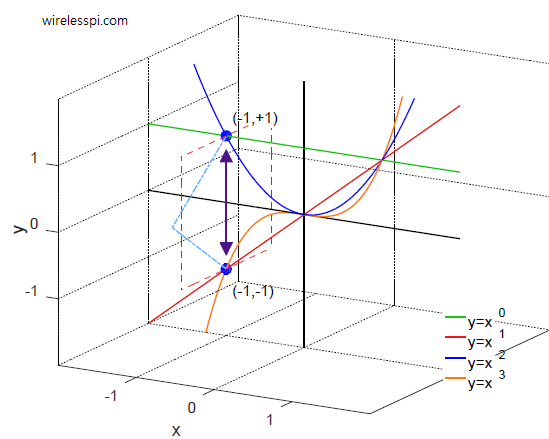
Figure 11: Plots for positive integer powers of $x$ in 3D

Now let us plot the integer powers of $x$ in 3D as in Figure 11. To reiterate, all the curves pass through $(+1,+1)$ for positive powers of $x$ but oscillate between the two points $(-1,+1)$ and $(-1,-1)$ for negative powers of $x$. This is shown below in the form of powers of $-1$.
\begin{align*}
(-1)^0 &= +1 \\
(-1)^1 &= -1 \\
(-1)^2 &= +1 \\
(-1)^3 &= -1 \\
\vdots
\end{align*}
This oscillation or vibration is represented by purple arrows in Figure 11. It is evident here that $+1$ on $x$-axis is a very dull number which does nothing noteworthy as an input to a function. On the other hand, $-1$ on $x$-axis is a very exciting number as an input to a function that heavily contributes to the beauty of mathematics, signals and our understanding of the universe. I will shed a little more light on this point in Section 8 on entering the world of DSP.

We infer the following requirements for the fractional powers of $x=-1$.

1. If $(-1)^0$ is $+1$ and $(-1)^1$ is $-1$, then the fractional powers of $-1$ must lie somewhere between $+1$ and $-1$. However, they cannot lie on $y$-axis due to the arguments leading to an empty left half for rational powers of $x$ in Figure 10. This necessitates that we depart the 2D plane and enter into an imaginary dimension, much like Platform $9\frac{3}{4}$ used for boarding the Hogwarts Express in the Harry Potter wizarding world. The dashed rectangle drawn in Figure 11 points towards this imaginary dimension coming out of the page. The fractional powers of $-1$ should lie somewhere here.



Figure 12: Platform $9\frac{3}{4}$ is the entry to an imaginary world

2. Starting from $(-1)^0$ at the top in Figure 11, the fractional powers of $-1$ must return to $(-1)^1$ at the bottom to maintain continuity. This is indicated by a half triangle in Figure 11. A journey from $(-1)^0$ to $(-1)^1$ also implies that the powers are uniformly distributed in this region and summation of two such powers while forming a product should simply move in proportion to this sum. For example,
   \[
   (-1)^{0.1}\cdot (-1)^{0.2} = (-1)^{0.1+0.2} = (-1)^{0.3}
   \]
   We conclude that $(-1)^{0.5}$ should lie on the corner of this triangle because $0.5$ lies in between $0$ and $1$. This is perpendicular to both $x$ and $y$ axis lines and represents the third dimension. From now onward, we will denote the original $y$-axis as $y_R$ while this new axis as $y_I$.
3. Owing to the properties of unity, the distance of each such point from $(x,y_R)$ $=$ $(-1,0)$, i.e., its length or magnitude, must be $1$. This implies that the fractional powers of $-1$ can lie neither on the rectangle nor on the triangle shown in Figure 11 because the lengths of all such points as measured from $(-1,0)$ will not be equal to 1. In which shape do all the points lie at an equal distance from its center? Yes, this must be a circle! The above discussion leads to the fractional powers of $-1$ lying on a circle in an imaginary dimension similar to a clock and shown in Figure 13.



Figure 13: Fractional powers of $-1$ are distributed on a circle similar to minutes of a clock

4. Finally, while the powers of $-1$ are uniformly distributed across the unit circle, what is uniformly spaced across the unit circle in 2D geometry? It is the angles! We conclude that the powers of $-1$ correspond to the angles across the unit circle, as shown on the right side of Figure 13. An immediate consequence of this is the following expressions.
   \begin{align*}
   (-1)^{0} \quad &\rightarrow \quad 0^{\circ} = 0 ~ \text{radians}\\
   (-1)^{0.5} \quad &\rightarrow \quad 90^{\circ} = \frac{\pi}{2} ~ \text{radians}\\
   (-1)^{1} \quad &\rightarrow \quad 180^{\circ} = \pi ~ \text{radians}\\
   (-1)^{1.5} \quad &\rightarrow \quad 270^{\circ} = \frac{3\pi}{2} ~ \text{radians}
   \end{align*}
   Since $(-1)^{0.5}$ lies on the perpendicular axis due to $0.5$ located exactly in the middle of $0$ and $1$, it is a rotation of the number $(-1)^0=1$ by $90^{\circ}$ in this 2D plane. Another implication of this perpendicularity is that we choose $(-1)^{0.5}$ as the representative member of the third dimension and give it a specific name: $i$.

By now, I have answered Question (a) from the list mentioned at the start of this guide: “What is the role of the number $\sqrt{-1}$? What sets it apart from other impossible numbers, e.g., a number $k$ such that $|k|=-1$?” To some extent, Question (b) is touched as well. Nevertheless, let us explore the answer to Question (b) in a little more depth.

5.2 Powers and Angles

---

With this understanding in place, we can quickly locate any power of $-1$ by traversing a path along this unit circle.
\begin{align*}
i^1 &= (-1)^{0.5} \\
i^2 &= (-1)^{(0.5)2} = (-1)^{1} = -1 \\
i^3 &= (-1)^{(0.5)3} = (-1)^{1.5} = (-1)^1 \cdot (-1)^{0.5} = -i \\
i^4 &= (-1)^{(0.5)4} = (-1)^{2} = +1 \\
\vdots
\end{align*}
We have already seen above how $i$ is a rotation of the number $1$ by $90^{\circ}$ in a 2D plane on a unit circle. Consequently, each subsequent power of $i$ (e.g., $i^2$) imparts a further $90^{\circ}$ rotation on the plane. After four such rotations, we return to the number $1$, as illustrated in Figure 14.

Figure 14: $i$ is a rotation of number $1$ by $90^{\circ}$ on a unit circle. Each subsequent power of $i$ rotates the result counterclockwise by a further $90^{\circ}$ until we return to $1$ for $i^4$

In this figure, I have incorporated the following two changes.

1. Departing from the 3D Figure 11, we have now moved the camera to the right and viewed the 2D plane made by $y_R$ (the real axis) and $y_I$ (the imaginary axis).
2. Initially I deliberately placed the starting angle $0$ or $(-1)^0$ at the top to portray how the number $i$ originated. Now I have drawn the plane made by $(y_R,y_I)$ in a regular fashion where the angle $0$ or $(-1)^0$ is placed at the right.

Now we can generalize the relationships between the powers of $-1$ and angles on a unit circle through Figure 15. For example, a power $0.1$ of $-1$ is traditionally written as $(-1)^{0.1}$ $=$ $0.95+0.31i$. In our simpler approach, this corresponds to
\[
0.5:90^{\circ}::0.1:? \qquad \Longrightarrow \qquad ? = \frac{90^{\circ} (0.1)}{0.5} = 18^{\circ}
\]
with a magnitude of $1$. As an extension, all multiples of $0.1$ correspond to multiples of $18^\circ$. This is illustrated in Figure 15 in the form of powers from $0$ to $1.9$ on the left and angles from $0^{\circ}$ to $342^{\circ}$ on the right.

Figure 15: Powers of $-1$ are distributed across the unit circle and $(-1)^{0.5}$ happens to lie between $0$ and $1$ on a perpendicular axis

In such a setup, we will have a summation of powers correspond to a summation of angles.
\begin{align*}
(-1)^{0.5} \quad &\Leftrightarrow \quad 90^{\circ}\\
(-1)^{0.2+0.3} \quad &\Leftrightarrow \quad 36^{\circ}+54^{\circ}
\end{align*}
This is how we move along the unit circle. This answers Question (b) from the list mentioned at the start of this guide: “Why is $\sqrt{-1}$ a rotation by $90^\circ$ in a 2D plane?” A square root and a rotation are related through this marriage of powers of $-1$ with angles.

5.3 A Great Mental Shift

---

Let us quickly recap the two biggest mental shifts one experiences in an understanding of imaginary numbers.

1. While the $x$-axis real line corresponds to the physical objects we come across (due to which you will never encounter imaginary numbers in the real world), nothing can be said about the $y$-axis real line. The mapping from $x$ to $y$ opens up the possibilities of discovering hitherto unknown crazy quantities, say imaginary, complex, figurative or convoluted numbers. This is in the nature of the problem: if you land on moon LV-426, you might run into Xenomorph XX121 instead of simple lifeforms similar to planet earth.

   

   But here is the good news: the confusion regarding $\sqrt{-1}$ and complex numbers is not due to an intellectual limitation of the learner. It is due to the way complex numbers are introduced by the masters.

2. There is a problem when complex numbers are introduced as a a point in a 2D plane as
   \[
   z = x+i\cdot y
   \]

   and shown as the blue plane in Figure 16. Such an introduction implies that a complex number $(x,y)$ is just one further extension to a real number $x$ by including $\sqrt{-1}$ on the vertical axis, a difficult concept to wrap your mind around. One wonders what is so special about $\sqrt{-1}$ that leads to devising a completely new category of numbers and placing $\sqrt{-1}$ on a perpendicular axis.

   

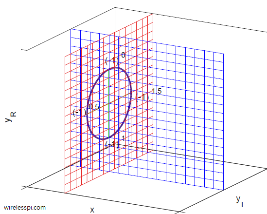
   Figure 16: A complex plane formed by a real and an imaginary axis

   In this alternative approach, any point in a 2D plane can be represented as a combination of multiples of $(-1)^0=1$ on real axis and multiples of $(-1)^{0.5}=i$ on imaginary axis because $i$ is simply a rotation of $90^{\circ}$ in a 2D plane ($0.5$ being in the middle of $0$ and $1$). Otherwise, power $0.5$ of $-1$ is not special in any other aspect.

   A complex number then is a point in a 2D plane formed by a real axis $y_R$ and an imaginary axis $y_I$ forming an ordered pair of numbers $(y_R,y_I)$. This is plotted as the red plane in Figure 16 where a unit circle at $x=-1$ is also drawn.
   \[
   z = (-1)^0 \cdot y_R + (-1)^{0.5}\cdot y_I = 1\cdot y_R + i\cdot y_I
   \]
   I feel a particular appreciation for this inclusion of $(-1)^0$ with the real part and $(-1)^{0.5}$ with the imaginary part (instead of $i$) because such a representation lays bare the whole concept of complex numbers right in the notation itself. Moreover, denoted as $(y_R,y_I)$ instead of $(x,y)$, it is evident that the real line $y_R$ came into being through operations on $x$-axis real line, and then functions involving powers gave rise to $y_I$ dimension.

6. Construction of the Curves

---

Recall that we encountered a missing left half plane for the fractional powers of $x$, see Figure 10. This was the question that took us to an exploration of the powers of $-1$ as rotations on the unit circle. We are now ready to fill the left half plane for the fractional powers of $x$, which is a little dissimilar to negative numbers filling the left half axis on the real line.

6.1 Generating $y=x^{0.5}$

---

Our first task is to draw the graph of $y=x^{0.5}$ for both positive and negative values of $x$. The traditional positive $x$ part was already plotted before but redrawn in the right half plane of Figure 17. For the negative half, assume as an example that $x=-0.3$. Then, we have
\[
(-0.3)^{0.5} = (-1 \times 0.3)^{0.5} = (-1)^{0.5}\cdot (0.3)^{0.5}
\]
We know the result for positive fractional power $(0.3)^{0.5}$ $=$ $0.548$, while we know the angle $(-1)^{0.5}$ as $90^{\circ}$ from the above discussion, see Figure 15. Consequently, we mark the point $(-0.3)^{0.5}$ with the same value as $(0.3)^{0.5}$ but at a $90^{\circ}$ angle from $y_R$ at $x=-0.3$ and shown with a green square in Figure 17. The conventional way to write such a point is $0.548i$.
\[
x =-0.3, \quad y_R = 0, \quad y_I = 0.548
\]

Figure 17: A complete graphical representation of $y=x^{0.5}$ including both positive and negative halves

Choose other negative values of $x$ and we have the complete curve for $y=x^{0.5}$ including both positive and negative halves and plotted in Figure 17, unlike the conventional graphical representation of $y=x^{0.5}$ that leaves the left half empty. Introducing an imaginary axis complements this positive half with a similar negative counterpart but at an orientation of $90^{\circ}$. The orange circle shown on the extreme left here is on the $(y_R, y_I)$ plane for $x=-1$, i.e., this is the same circle drawn before in Figure 15. That is why we can see the powers of $-1$ in the form of angles of $0^{\circ}$, $90^{\circ}$, $180^{\circ}$ and $270^{\circ}$ in their respective positions. As a reminder, $0^{\circ}$ is at the top because our focus is to illustrate the origins of $-1$ powers, otherwise a conventional complex plane pins $0^{\circ}$ at the right. Finally, the blue dot at the left end is the point $(-1)^{0.5}$ where the curve $x^{0.5}$ naturally cuts through at $x=-1$. I find such a figure as pleasing to the mind as a scenic mountain.

6.2 Generating Fractional Powers

---

From the above discussion, a general algorithm to draw the negative half for any fractional power $x^f$ can be written as follows.

1. Choose a negative value for $x$.
2. Find the outcome $x^f$ by writing $x$ as a product of $-1$ and a positive fractional number.

   \[
   x^f = (-1\cdot |x|)^f = (-1)^f\cdot |x|^f, \qquad \qquad x<0 \]

3. Here, $(-1)^f$ provides the angle as picked up from Figure 15 while the positive fractional number $|x|^f$ provides the magnitude. Together, they locate a point in a 3D plane formed by $x$, $y_R$ and $y_I$.
4. Repeat for other negative values of $x$ and join all such points for creating the final graph.

Our next step is to draw similar curves for any other fractional power of $x$ including the negative half, some examples of which are illustrated in Figure 18. This becomes straightforward by utilizing the algorithm above. We will locate each point through a combination of angle from the power of $-1$ and magnitude from the remaining positive fraction.

Figure 18: A complete graphical representation of fractional powers of $x$ including both positive and negative halves

As an example, suppose that the required graph is that of $y=x^{0.2}$. Then, for one particular value of $x$, say $-0.3$ again, we can write
\[
(-0.3)^{0.2} = (-1 \times 0.3)^{0.2} = (-1)^{0.2}\cdot (0.3)^{0.2}
\]
We know the result for positive fractional power $(0.3)^{0.2}$ $=$ $0.786$, while we know the angle $(-1)^{0.2}$ as $36^{\circ}$ from the above discussion, see Figure 15. Consequently, we mark the point $(-0.3)^{0.2}$ with the same value as $(0.3)^{0.2}$ but at a $36^{\circ}$ angle from $y_R$ at $x=-0.3$ shown with an orange square in Figure 18. Due to the 2D plane formed by $y_R$ and $y_I$ blended with the principles of geometry, this point turns out to be
\[
x =-0.3, \quad y_R = 0.786 \cdot \cos 36^{\circ} = 0.636, \quad y_I = 0.786 \cdot \sin 36^{\circ} = 0.462
\]
The conventional way to write such a point is $0.636+0.462i$. Choose other negative values of $x$ and we have the complete curve for $y=x^{0.2}$ including both positive and negative halves illustrated in a green color in Figure 18. Moreover, the curves for some other fractional powers of $x$, i.e., $y=x^{0.7}$ and $y=x^{1.3}$, are also drawn for further clarity in red and light blue colors, respectively. For each such curve, notice how the power of $-1$ provides the angle at which the ensuing graph is located. To find the exact angle, refer to Figure 15 where $(-1)^{0.7}=126^{\circ}$ and $(-1)^{1.3}=234^{\circ}$.

In Figure 18, all three curves lie on the real $y$-axis at $0^{\circ}$ for the positive $x$-axis. For the negative $x$-axis, I have shown the three curves from a particular camera angle emerging from origin and going towards their respective amplitudes at different angles, namely, $36^{\circ}$, $126^{\circ}$ and $234^{\circ}$. If the angle information is taken out, then there is no difference between the positive and negative halves and a symmetry is achieved that is coming next.

To sum it up, the fractional powers of $x$ $=$ $0.25$, $0.50$, $0.75$, $1.00$, $1.25$ and $1.50$ are arranged in a circle in the plots of Figure 19a. To set our reference, observe that the red curve for $y=x^{0.5}$ is the same as previously shown in Figure 17 while the orange line is the familiar $y=x^1$ graph. All the graphs are located at angles corresponding to their powers of $-1$ and are uniformly spaced across the unit circle due to their chosen values (all are multiples of $0.25$). Trace each and every of these curves in a circle starting from $0.25$, ending on $1.50$ and cutting through the orange unit circle in a counterclockwise manner and it will surely delight your heart.

Figure 19a: Fractional powers of $x$ $=$ $0.25$, $0.5$, $0.75$, $1$, $1.25$ and $1.75$ arranged around the unit circle in the negative half

Figure 19b: Magnitude plots $|y|$ for curves on the left with circles on $(-1,+1)$ and $(+1,+1)$, exhibiting an even symmetry beautifully crafted through imaginary numbers

The next step is to form the magnitude plots depicting this beautiful symmetry. If you are reading these lines on a color screen, you can compare the colors of the curves in 3D plane of Figure 19a with 2D plane of Figure 19b drawing the magnitude plots. I find this symmetry arising from our own choice of numbers quite extraordinary, just like the bilateral symmetry exhibited by moving creatures (e.g., your two legs) arising due to gravity that helps them smoothly turn in both directions. In particular, the negative half on $y$-axis in Figure 19b complements the positive half in a similar manner as negative half on the $x$-axis complements the positive half in the case of negative numbers.

Now I am going to use almost the same sentences in the next two lines that I used at end of the section on negative numbers: To cater for the corner case where fractional powers of $x$ are only defined for the positive half, an innovation in the form of imaginary numbers was introduced by assigning an angle as a power of $-1$ in an extra dimension to a real number. And so imaginary numbers made it possible to establish symmetrical counterparts to fractional powers of positive $x$ on the same plane.

This reminds me of the words from Alan Lightman on symmetry:

This is time we move towards answering the last question in our list on the role of the mathematical constant $e=2.71828$ in this picture.

7. Role of the Constant $e$

---

To keep the article length short, I have answered this question in detail in a separate post Why the constant e arises in complex plane as a rotation.

8. Door to the World of DSP

---

According to Nikola Tesla: "If you want to find the secrets of the universe, think in terms of energy, frequency and vibration." It has been known that everything in the universe is constantly vibrating or oscillating at a certain frequency. To decode the secrets of the frequencies in the universe, the field of DSP defines some fundamental signals associated with such oscillations, as we see next.

Let us recall Figure 11 now where we plotted the integer powers of $x$ in 3D. In that figure, all the curves pass through $(+1,+1)$ for positive powers of $x$ but oscillate between the two points $(-1,+1)$ and $(-1,-1)$ for negative powers of $x$ which was represented by purple arrows. Now we will associate the variable time denoted by $t$ with each such power.
\begin{align*}
t=0 \qquad \rightarrow \qquad (-1)^0 &= +1 \\
t=1 \qquad \rightarrow \qquad (-1)^1 &= -1 \\
t=2 \qquad \rightarrow \qquad (-1)^2 &= +1 \\
t=3 \qquad \rightarrow \qquad (-1)^3 &= -1 \\
\vdots
\end{align*}
From the above expressions, we can construct a signal $s(t)$ as
\[
s(t) = (-1)^t
\]
which is plotted in Figure 26. Observe that the signal is defined only for integer values of $t$ and there are no real values in between two such integers. The signal is constantly vibrating between $+1$ and $-1$ marked by red crosses at each time instant.

Figure 26: Oscillations arising from $s(t)=(-1)^t$ at discrete time intervals

Since we have figured out the graphs for fractional powers of $x$, we know that there are no jumps here and the values of the fractional powers fill the space in between such samples (we now know exactly what $(-1)^{0.5}$ or $(-1)^{1.67}$ mean, for example). This is consistent with other natural processes, most (but not all) of which are continuous functions. These fractional powers of $x$ lie on a unit circle encompassing $+1$ and $-1$ with each point lying at a distance of unity, as shown previously in Figure 15. When we stretch such a circle in time domain (not $x$-axis), it starts coming out of the page in the form of rotations as illustrated in Figure 27a. The red crosses marking $+1$ and $-1$ on this 3D curve are still visible. One such rotation takes $2$ time units as
\[
(-1)^0 = (-1)^2 = +1
\]
This gives rise to a spiral shape with changeable frequencies that forms the fundamental set of signals employed for the analysis and synthesis of real-world signals. Such a shape that fills the space between $+1$ and $-1$ with the fractional powers of $-1$ is very similar to a slinky toy that is stretched to form a spiral in Figure 27b.

Figure 27a: Oscillations arising from $s(t)=(-1)^t$ at a continuous time scale form a complex sinusoid $s(t)=e^{i\omega t}$ which is the fundamental signal in DSP

Figure 27b: Stretching the oscillations from $(+1,-1)$ is similar to stretching a slinky toy

What do you think is the mathematical form of this signal? It is the same $s(t) = (-1)^t$ with the difference that $t$ is now a continuous variable of time and not an integer only. From the most beautiful equation in mathematics, we know that $-1=e^{i \pi}$. Therefore, the equation for such a rotating spiral is
\[
s(t) = (-1)^t = e^{i \pi t}
\]
Comparing with the standard frequency of any oscillation, we get
\[
2\pi Ft = \pi t \qquad \rightarrow \qquad F = \frac{1}{2}
\]
which makes sense because we saw earlier that one rotation in a circle starting and ending at $(-1)^0=+1$ completes in $T=2$ time units. For a general frequency $2\pi F = \omega$, this signal becomes
\[
s(t) = e^{i\omega t}
\]
which is commonly known as a complex sinusoidal signal. From Euler’s identity, we can break a complex sinusoid in real and imaginary parts as
\[
s(t) = e^{i\omega t} = \cos \omega t + i\cdot \sin \omega t
\]
These real and imaginary components are also plotted in Figure 27a on the floor and the wall depicting the real and imaginary planes, respectively. This complex sinusoid forms the basis of the Fourier Transform, about which it is often said that one needs four years to understand the concept. Nevertheless, with this background, I hope that you can learn the fundamentals of DSP in a much shorter time.

---