Goertzel Algorithm – Evaluating DFT without DFT

The Discrete Fourier Transform (DFT) computes the contribution of $N$ sinusoids that come together to form any input signal. However, in some applications, we are only interested in contributions from one or a few sinusoids This is where the Goertzel algorithm, proposed by Gerald Goertzel in 1958, comes in.

The Goertzel algorithm evaluates the individual terms of the DFT in an efficient manner. We explain its derivation and implementation with the help of DTMF signals.

DTMF Signal Generation

In the early days of telephone, you could not call anyone directly. Instead, a telephone operator used to sit on the other side of the line. Whenever you picked up the phone, you told the operator where to connect and they manually relayed your call on a central switchboard.

This was not going to last. People need to connect to a lot of people beyond the capacity of this kind of system. A control signaling mechanism for automatic routing was the answer.

Dual Tone Multi-Frequency (DTMF) signals were designed to send the control signals (e.g., the destination phone number or a particular number) within the voice band. Their significance decayed with time due to separate control channels in cellular transmissions but their association with the keypad has kept them alive for many applications today. Examples are customers navigating a telephone menu of a company, responding to certain questions by pressing the buttons on the dial pad and entering credit card or account details for a phone transaction.

Let us start with a keypad as shown in the figure below.

In DTMF, there are 4 tones in a low group of frequencies (corresponding to each row of the keypad above).
\[
697, 770, 852, 941 \quad \text{Hz}
\]

In addition, there are 4 tones in a high group of frequencies (corresponding to each column in the keypad above).
\[
1209, 1336, 1477, 1633 \quad \text{Hz}
\]

The last column showing letters A through D are missing in the above figure because they are rarely used.

Each key press generates two tones, or sinusoids: one from the low frequency group (row) and the other from a high frequency group (column). For example, pressing the number 6 generates a sum of two sinusoids, one at 770 Hz and the other at 1477 Hz.

Python code to generate the above signals is given below. If you work in Maltab/Octave, you can also read about how to generate a sinusoid and view its spectrum.

import numpy as np
import matplotlib.pyplot as pl

figWidth = 8
figHeight = 6

# Parameters

rowtones = np.array([697, 770, 852, 941]);
coltones = np.array([1209, 1336, 1477]);

keytones = [[[rowtones[i], coltones[j]] for j in range(3)] for i in range(4)]

# Signal Generation

fs = 24e3 # sample rate
Ts = 1/fs; # sample time

mykey = keytones[1][2] # Key 6

T = 0.02;

t = np.arange(0, T, Ts)
A = 2
phi = 0*np.pi/180

x1 = A*np.sin(2*np.pi*mykey[0]*t + phi)
x2 = A*np.sin(2*np.pi*mykey[1]*t + phi)
x = x1+x2

# Plotting the signal

fig, axs = pl.subplots(3, figsize=(figWidth, figHeight))

axs[0].plot(t,x1,linewidth=2,color='b')
axs[1].plot(t,x2,linewidth=2,color='r')
axs[2].plot(t,x,linewidth=2,color='g')

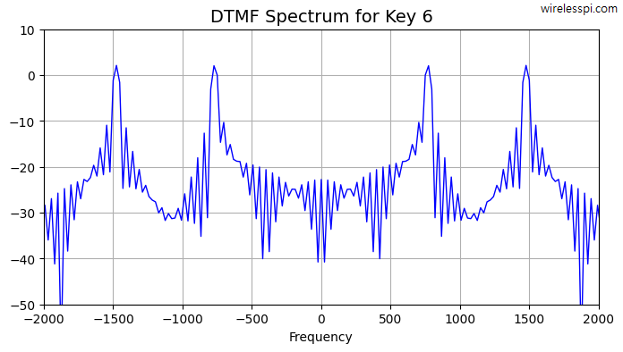
The spectrum of this signal can be viewed through the FFT command and drawn in the figure below. Clearly, the two spikes at $\pm 770$ Hz and $\pm 1477$ Hz indicate the presence of the two tones corresponding to key 6.

Notice in the above figure that computational complexity of taking a Discrete Fourier Transform (DFT) is high due to $N$ frequencies involved. In many applications such as spectral analysis and wireless communications, this is exactly what is needed. However, in applications like DTMF detection, an efficient evaluation of a small number of known frequency components is required.

This is why we now move towards Goertzel algorithm for detection of particular tones in a signal.

DTMF Signal Detection – The Goertzel Algorithm

As described above, the Goertzel algorithm is a method even faster than the Fast Fourier Transform (FFT) for detection of a tone with a particular frequency in a signal. There is no magic: this is accomplished by focusing only on one target frequency and ignoring the rest of the DFT output.

Time Domain Recursion

The starting point is the definition of the Discrete Fourier Transform (DFT).
\[
X[k] = \sum_{n=0}^{N-1} x[n]e^{-j2\pi \frac{k}{N}n}, \qquad k = 0,1,\cdots,N-1
\]

It is evident from the above expression that the index $k$ goes from $0$ to $N-1$ too. For a fixed $k=k_0$, the Goertzel algorithm works as follows.

For $k=k_0$, we can multiply both sides with $e^{j2\pi \frac{k_0}{N}N}$ because $e^{j2\pi k_0}=\cos 2\pi k_0+ j\sin 2\pi k_0=1$ for any $k_0$.
\[
X[k_0] = \sum_{n=0}^{N-1} x[n]e^{j2\pi \frac{k_0}{N}(N-n)}
\]

The right side looks similar to a convolution sum at time $N$ between two signals, $x[n]$ and $e^{j2\pi \frac{k_0}{N}n}$. This can be written as
\[
\begin{aligned}
X[k_0] = x[0]e^{j2\pi \frac{k_0}{N}(N-0)} + x[1]e^{j2\pi \frac{k_0}{N}(N-1)}&+x[2]e^{j2\pi \frac{k_0}{N}(N-2)} \\&+ \cdots + x[N-1]e^{j2\pi \frac{k_0}{N}\{N-(N-1)\}}
\end{aligned}
\]

Clearly, $x[0]$ is multiplied with $e^{j2\pi \frac{k_0}{N}}$ a total of $N$ times, $x[1]$ is multiplied with the same term $N-1$ times, while $x[N-1]$ is multiplied only 1 time. The expression can now be simplified as
\[
X[k_0] = \left[\cdots\left[\left[\underbrace{x[0]e^{j2\pi \frac{k_0}{N}} + x[1]}_{y_1}\right]e^{j2\pi \frac{k_0}{N}}+x[2]\right]e^{j2\pi \frac{k_0}{N}} \cdots + x[N-1]\right]e^{j2\pi \frac{k_0}{N}}
\]

This gives rise to the following recursion.
\[
\begin{aligned}
y_0 &= x[0] \\
y_1 &= y_0e^{j2\pi \frac{k_0}{N}} + x[1] \\
y_2 &= y_1e^{j2\pi \frac{k_0}{N}} + x[2] \\
\vdots ~&= \quad \vdots
\end{aligned}
\]

In summary, the recursion proceeds as follows.
\[
y_n = y_{n-1}e^{j2\pi \frac{k_0}{N}} + x[n]
\]

There is no efficiency gain visible yet. For this purpose, we need to go into complex frequency or z-domain.

The Two Filters

Taking the z-Transform of both sides of the last equation and using the time delay property, we get
\[
Y(z) = e^{+j2\pi \frac{k_0}{N}}\cdot z^{-1}Y(z) + X(z)
\]

This can be written as
\[
\frac{Y(z)}{X(z)} = \frac{1}{1-e^{+j2\pi \frac{k_0}{N}}z^{-1}}
\]

Now we divide and multiply by the conjugate term that separates the filter into two parts.
\[
\frac{Y(z)}{X(z)} = \frac{1-e^{-j2\pi \frac{k_0}{N}}z^{-1}}{\left(1-e^{+j2\pi \frac{k_0}{N}}z^{-1}\right)\left(1-e^{-j2\pi \frac{k_0}{N}}z^{-1}\right)}
\]

Let us create an intermediate signal $v_n$ with a z-Transform $V(z)$. Then, we have
\begin{equation}\label{equation-fir-iir}
\frac{Y(z)}{V(z)}\cdot \frac{V(z)}{X(z)} = \left(1-e^{-j2\pi \frac{k_0}{N}}z^{-1}\right)\cdot \frac{1}{\left(1-e^{+j2\pi \frac{k_0}{N}}z^{-1}\right)\left(1-e^{-j2\pi \frac{k_0}{N}}z^{-1}\right)}
\end{equation}

Consequently, the recursion $y_n$ is generated from $v_n$ through the inverse z-Transform of the first term above.
\[
\frac{Y(z)}{V(z)} = \left(1-e^{-j2\pi \frac{k_0}{N}}z^{-1}\right)
\]

In time domain, this yields the Finite Impulse Response (FIR) filter term.
\begin{equation}\label{equation-goertzel-fir}
y_n = v_n ~-~ e^{-j2\pi \frac{k_0}{N}}\cdot v_{n-1}
\end{equation}

Here, we produced $y_n$ from the intermediate signal $v_n$. On the other hand, the signal $v_n$ is generated from the input $x[n]$ through the second term in Eq (\ref{equation-fir-iir}) above.
\[
\begin{aligned}
\frac{V(z)}{X(z)} &= \frac{1}{\left(1-e^{+j2\pi \frac{k_0}{N}}z^{-1}\right)\left(1-e^{-j2\pi \frac{k_0}{N}}z^{-1}\right)} \\
&= \frac{1}{1-2\cos \left(2\pi \frac{k_0}{N}\right) z^{-1} + z^{-2}}
\end{aligned}
\]

where we have used the Euler’s identity $2\cos \theta$ $=$ $e^{+j\theta}+e^{-j\theta}$ above. Next, collect $V(z)$ and $X(z)$ terms on each side.
\[
V(z)\left[ 1-2\cos \left(2\pi \frac{k_0}{N}\right) z^{-1} + z^{-2}\right] = X(z)
\]

In time domain, this produces the Infinite Impulse Response (IIR) filter term as
\begin{equation}\label{equation-goertzel-iir}
v_n = 2\cos \left(2\pi\frac{k_0}{N}\right) v_{n-1} ~-~ v_{n-2} \,+\, x[n]
\end{equation}

The FIR Eq (\ref{equation-goertzel-fir}) and IIR Eq (\ref{equation-goertzel-iir}) can now be combined for the complete algorithm.

With the output in hand, you can take the magnitude for all 7 frequencies and decide whether the target frequency is present or not based on a threshold value.

You can use the code below in Python to detect the magnitudes of DTMF tones in a given signal.

N = len(x)
mags = [0]*7
tones = np.concatenate((rowtones, coltones))
print(tones)

for fcount in range(7):
  k0 = N*tones[fcount]/fs # check the article on discrete frequency for this step

  omega_I = np.cos(2*np.pi*k0/N)
  omega_Q = np.sin(2*np.pi*k0/N)
  v1 = 0
  v2 = 0
  for n in range(N):
    v  = 2*omega_I*v1 - v2 + x[n] # see the IIR Eq (3)
    v2 = v1
    v1 = v
  
# Now value of v is in v1 and that of v1 is in v2
  y_I = v1 - omega_I*v2 # see the FIR Eq (2)
  y_Q = omega_Q*v2
  
  mags[fcount] = y_I**2 + y_Q**2 # figure below plotted after square root

When the code above is run for the signal corresponding to key 6 generated earlier in this article, the output is shown in the figure below. It is clear that the two frequencies $770$ Hz and $1477$ Hz are present in the signal thus leading to the result that key 6 was pressed at the other end of the line.

We now describe why the algorithm is so efficient.

Efficiency

The efficiency in the above code appears as follows.

• In the FIR Eq (\ref{equation-goertzel-fir}), only $\cos(2\pi k_0/N)$ and $\sin(2\pi k_0/N)$ terms are required. This saves memory in the embedded system.
• In the IIR Eq (\ref{equation-goertzel-iir}), only one constant coefficient, namely $2\cos(2\pi k_0/N)$, is required. This multiplication by 2 can be simply implemented by a left shift of the cosine term above, thus allowing to compute the coefficient in real-time. Also, the other coefficient is just $1$.
• The signal duration and sample rate determine the data length $N$. Among the available options, the best choice comes from the relation
  \[
  k_0 = \frac{f}{f_s}N
  \]

  such that DTMF frequencies are as close to bin center as possible to avoid the scalloping loss. The interesting point is that unlike FFT, the length $N$ does not have to be a power of 2.

• As evident from the code above, the loop runs the IIR part. The FIR part is only computed once after $N$ samples.
• A threshold level to differentiate between presence or absence of a tone can be determined through an empirical investigation of the system.
• A window might be required for the data sequence to avoid the leakage problem.

Optimized Goertzel Algorithm

The IIR part of the Goertzel algorithm is run $N$ times and the FIR part only once. Observe that both the real and imaginary parts are computed in the FIR filter Eq (\ref{equation-goertzel-fir}). If the phase information is sacrificed, an optimized algorithm can combine the last three steps in one operation to speed up the processing time.

Since $\cos^2\theta+\sin^2 \theta=1$, we have the magnitude squared altered as follows.

# Instead of
  y_I = v1 - omega_I*v2
  y_Q = omega_Q*v2

  mags[fcount] = y_I**2 + y_Q**2

# Use  
  mags[fcount] = v1**2 + v2**2 -2*omega_I*v1*v2