Two Birds with One Tone: I/Q Signals and Fourier Transform – Part 2

Let us start with a new perspective that will lift more veils from the I/Q puzzle.

A Basic Building Block

Humans use the power of logic to uncover the rules according to which the world works. But our minds struggle to retain excessive amounts of information required to grasp the complex reality. Therefore, we like to reduce everything around us as a combination of some fundamental unit, a concept known as reductionism.

Some examples of reductionism are

• atoms in all matter,
• cells in living organisms,
• bits in digital information,
• pixels in digital images,

and so on.

The opposite view is that of emergence: an entity is more than the sum of its parts. As most of us have experienced, two kids together are much naughtier than summation of either one alone 🙂 Fortunately, the world of linear signals and systems is reductionist, not emergent.

Humans seek basic structural and functional units because we are suckers for compactness. This simplifies our understanding of the world, allows us to analyze phenomena more effectively and make informed decisions. In the real world, for instance, the government employs the basic unit of money to allocate budget for education, health, defense, and the likes.

Are electronic signals also made up of combinations of a fundamental signal?

The Fundamental Signal

Just like atoms, cells, bits and pixels in the above example, we seek an elemental component of signals. As it turns out, our old friend, the sinusoid, plays a new role in this regard.

Sinusoids: A New Role

Consider a common example of our 3D space where the vectors x, y and z are orthogonal to each other.

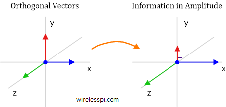
Any point in this 3D space can be written as a combination of the basis vectors with x, y and z coordinates.
\[
\mathbf{r} = x \mathbf{i} + y\mathbf{j}+ z\mathbf{k}
\]

where $\mathbf{i}$, $\mathbf{j}$ and $\mathbf{k}$ are the unit vectors in those dimensions.

Is there something similar in the world of signals? We presume that a sinusoid, the smoothest of signals, can act as such a basic unit. This idea can be seen in the figure below that plots four sinusoids with different frequencies.

When we sum these four signals, the result is a waveform that resembles a square wave, as illustrated by blue and red lines in the figure below. Increasing the number of sinusoids in a similar manner refines the approximation.

If even a signal with sharp corners like a square wave can be approximated by the sum of sinusoids, this means that the idea of viewing them as basic building blocks is a path worth exploring (this path reveals a hidden strategy at play since the frequencies and amplitudes of the above sinusoids were not randomly chosen).

Now a simple sinusoidal signal has the expression
\[
x(t) = A \cos (\omega t + \phi)
\]

where $A$ is the amplitude, $\omega$ is the angular frequency and $\phi$ is the phase shift.

We saw in Part 1 that with a sum of elementwise products (a numerical prism commonly known as the dot product),

• orthogonality in amplitude is not possible, and
• orthogonality in phase generates two possible carrier waves, one in $I$ arm and the other in $Q$ arm.
  \[
  \begin{aligned}
  I(t) &= \cos \omega t\\
  Q(t) &= -\sin \omega t
  \end{aligned}
  \]

• Continuing in this manner and viewing this sinusoid as a basis signal, the final turn is that of orthogonality in frequency. However, it is not clear that this orthogonality in frequency should be examined with
  • two cosines of different frequencies,
  • two sines of different frequencies, or
  • a combination of cosine and sine.

All three options above are possible but for reasons beyond the scope of this article, we focus on the last one. Since cosine and sine signals are mutually orthogonal in phase shift, they can be unified within a single framework by going into a higher dimension.

Flatland: A Romance of Many Dimensions

In 1884, an English schoolmaster Edwin Abbott Abbott wrote a satirical story Flatland: A Romance of Many Dimensions about a 2D world inhabited by geometric figures. In the story, a Sphere visits a Square in Flatland but the Square can only perceive it as a circle. The Sphere moves up and down, showing the Square how the circle changes size but the Square still cannot grasp the concept (imagine sunrise in a 2D world).

Before we get too confident about our mental faculties and perceive the Flatlanders as inferior beings, do we really understand the idea of higher dimensions ourselves? Looking at the figure above, I often ask myself if we can use a 2D paper/screen to draw 3D shapes, why can we not easily visualize 4D shapes from their 3D projections around us? To me, it certainly feels that 3 dimensions close the spatial loop but then maybe 2D beings also feel the same and we are all equal in our respective dimensional worlds.

Having said that, it is true that many ideas become clear only by going one level up from where we are standing. That is why we go from 1D to 2D world of DSP.

A Complex Sinusoid

In Flatland, the social status of a geometric figure is determined by the number of its sides. The circle, with its infinite sides, is considered the perfect shape. Let us investigate what happens when a path is traced along this perfect shape.

Consider the tip of a complex number (shown in blue below) at $x=1$ and assume that it starts rotating in counterclockwise direction with time. This implies that its angle also starts increasing at a rate of $\omega$ radians/second and given by
\[
\theta = \omega t
\]

As this motion generates a circle in a 2D-plane, we can observe its projection onto the horizontal axis by holding a torch at the top-down viewpoint. This is illustrated in the figure below.

Observe the green square above. As the complex number rotates around the unit circle, the green square starts at 1 and then oscillates on the x-axis from right to left and back. From simple trigonometry, this horizontal projection is a cosine wave!
\[
\begin{align*}
\text{Horizontal projection} &= \cos (\omega t)\\\\
\text{Vertical projection} &= \sin (\omega t)
\end{align*}
\]

In a similar manner, holding the same torch at a right-left viewpoint, we can observe the projection of this circular motion onto the vertical axis. The red diamond starts at zero and then oscillates on the y-axis in a top-down manner. It is clear that this vertical projection is a sine wave.

Some people find moving signals easier to understand. Hence, I made the animation below to demonstrate how a circular motion projects a cosine and a sine on each axis. The trick here is to observe only one square, either red or green, within the circle for some amount of time.

A visualization of circular motion projecting cosine and sine

If you think that all of the above is some clever math or theory, time to reconsider. Recall from Part 1 here that a complex DC signal can be seen on an oscilloscope. When this red square starts rotating in an anticlockwise direction, i.e., $\sin (\omega t)$ is plotted against $\cos(\omega t)$ for a frequency $\omega$, the result is shown on an oscilloscope in the figure below (for DSP folks looking very carefully, I could not find a good oscilloscope image with both probes connected :)).

When viewed in 3D, this rotating complex number traces the fundamental signal in DSP, known as a complex sinusoid with the frequency $\omega$. This is illustrated in the figure below.

The real or $I$ part of this complex sinusoid is $\cos \omega t$ and the imaginary or $Q$ part is $\sin \omega t$. This suggests that, rather than dealing with two distinct real sinusoids, we now encapsulate them within a single complex entity.

The Euler’s formula mathematically describes this signal as
\begin{equation}\label{equation-complex-sinusoid}
e^{j\omega t} = \cos(\omega t) + j\sin(\omega t)
\end{equation}

In this framework, negative frequencies also exist.

Negative Frequency

Just like it was difficult to accept negative numbers, negative frequencies do not make sense as an inverse period ($f=1/T$). But in an I/Q plane, a complex sinusoid rotating in a clockwise direction is given by $e^{-j\omega t}$ where a negative frequency, $-\omega$, indicates a clockwise rotation. Simply assume the red square on the oscilloscope above rotating in the opposite direction, i.e., $-\sin(\omega t)$ plotted against $\cos(\omega t)$ here.

\begin{equation}\label{equation-negative-frequency}
e^{-j\omega t} = e^{j(-\omega)t} = \cos (\omega t)\, – j \sin (\omega t)
\end{equation}

This complex sinusoid with a negative frequency is plotted in the figure below.

Next, we explore how these fundamental signals give rise to the frequency domain.

Frequency Domain

We usually think of frequency in terms of vibrations (number of cycles/second). But frequency domain is formally defined in terms of number and direction of rotations. There are no natural laws involved here, just human convention.

In frequency domain, a complex sinusoid rotating anticlockwise with a frequency $F$ is a single impulse at $F$. This is plotted in the figure below. In terms of angular frequency $\omega$, this would be at $\omega = 2\pi F$.

A unit impulse $\delta(\omega)$ is an ideal signal with width $\Delta \rightarrow 0$ and height $1/\Delta \rightarrow \infty$ such that
\[
\text{Area under the rectangle} = \Delta \cdot \frac{1}{\Delta} = 1
\]

On a similar note, a complex sinusoid rotating clockwise with a frequency $F$ is a single impulse at $-F.$ In the above figure, observe the direction of rotation of the sinusoids and the corresponding positive and negative frequency impulses.

In general, when a signal is drawn in frequency domain, the graph actually shows the $I$ and $Q$ amplitudes of those complex sinusoids whose frequencies are present in that signal. For example, consider the figure below with two complex sinusoids: $e^{j\omega t}$ shown as blue line while $e^{-j\omega t}$ shown as red line. Their $I$ and $Q$ components are similarly drawn as blue and red lines, respectively.

• The $I$ parts exactly fall on top of each other and hence are the same signal $\cos (\omega t)$.
• The $Q$ parts carry exactly the same amplitude with opposite signs to each other and hence are $\sin(\omega t)$ and $-\sin (\omega t)$, respectively.

Notice from the above figure that when two such complex sinusoids are added together, the $I$ parts add up point-by-point while the $Q$ arms cancel out as a result of this addition.

This can be mathematically seen from adding Eq (\ref{equation-complex-sinusoid}) and Eq (\ref{equation-negative-frequency}).
\[
e^{j\omega t} + e^{-j\omega t} = 2\cos (\omega t) \quad \implies \cos (\omega t) = \frac{1}{2}e^{j\omega t} + \frac{1}{2}e^{-j\omega t}
\]

This means that a cosine wave (having all the waveform on real axis in time domain and no imaginary component) has a frequency domain representation, known as its spectrum, that consists of two impulses. This frequency domain representation or spectrum of a cosine wave is illustrated in the figure below.

• One impulse is at frequency $\omega$ (or $F$ in Hz) with an amplitude of $1/2$.
• The other impulse is at $-\omega$ (or $-F$ in Hz), again with an amplitude of $1/2$.

The spectrum of a sine wave can also be drawn in an analogous manner. We can use both Eq (\ref{equation-complex-sinusoid}) and Eq (\ref{equation-negative-frequency}) to arrive at
\[
e^{j\omega t}\, – e^{-j\omega t} = j2\sin (\omega t) \quad \implies \sin (\omega t) = \frac{j}{2}e^{-j\omega t}\, – \frac{j}{2}e^{j\omega t}
\]

where we have used the property $j^2=-1$ to get
\[
\frac{1}{j} = \frac{j}{j^2} = -j
\]

To understand the above figure, use Euler’s identity again due to which we can write
\[
e^{-j\pi/2} = \cos (\pi/2)\, – j\sin (\pi/2) = 0\, – j\cdot 1 = -j
\]

In words, a multiplication by $-j$ is the same as a rotation by a phase angle $-\pi/2$ or $-90^\circ$. Therefore, in the above figure, observe how both impulses in the top figure are rotated clockwise by $90^\circ$ to arrive at the bottom figure.

The next logical step is to explore where orthogonality in frequency leads us.

Orthogonality in Frequency

Many such sinusoids come together to form a signal and the width they occupy on frequency axis is known as bandwidth. To see this idea, let us start with two complex sinusoids stored in digital memory with different frequencies but same amplitude and phase shift.

• Without loss of generality, we assume that the amplitude $A=1$ and phase shift $\phi=0$.
• Also, just like real correlation multiplies two signals elementwise, a complex correlation can correspond to a similar result if the second signal has a complex conjugate (i.e., negative of the original phase) to suppress the phase and multiply the magnitudes.

Then, over a period $\tau$, we can write
$$\begin{equation}
\begin{aligned}
r = \int _{-\tau/2}^{\tau/2} e^{j\omega_1 t}\cdot e^{-j\omega_2 t}dt &= \int_{-\tau/2}^{\tau/2} e^{j(\omega_1 – \omega_2) t}dt\\\\
&= \frac{e^{\left[j(\omega_1 – \omega_2) t\right]}}{j(\omega_1-\omega_2)}\Bigg|_{-\tau/2}^{\tau/2}
\end{aligned}
\end{equation}\label{equation-orthogonality}
$$

Let us use the symbol $\Delta = \omega_1 – \omega_2$. This results in
\[
r = \frac{1}{j\Delta_\omega}\left[e^{j\Delta_\omega \tau/2} – e^{-j\Delta_\omega \tau/2}\right]
\]

From Euler’s formula, we have $\sin\theta$ $=$ $(e^{j\theta}-e^{-j\theta})/2j$. Plugging in the above expression, we get
\[
r = 2\frac{\sin \left(\Delta_\omega \tau/2\right)}{\Delta_\omega}
\]

In signal processing, a sinc signal is defined as
\[
\text{sinc} (x) = \frac{\sin (\pi x)}{\pi x}
\]

Using $\Delta_\omega = 2\pi \Delta_f$, we can modify our last expression as
\begin{equation}
r = \frac{\sin (\pi\; \tau\Delta_f)}{\pi \Delta_f} = \tau~ \text{sinc} (\tau\Delta_f)\label{equation-dot-product-result}
\end{equation}

where $\Delta_f= f_1-f_2$. This expression is plotted in the figure below for $\tau=1$.

To summarize, we compute the dot product between two signals. If the result is zero, they are orthogonal to each other.

• In the case of amplitude, we found that it was impossible to achieve orthogonality.
• In the case of phase shift, we found only two waves orthogonal to each other.
• Here in the case of frequency, we have a strange looking sinc curve as a result of the dot product. How to make sense out of this graph?

The Fourier Transform

The dot product between complex sinusoids in the above figure was plotted for integration period $\tau=1$. Let us examine the above result for $\tau$ $\rightarrow$ $\infty$, i.e., for an infinitely long duration of time.

It is clear from the above figure that as $\tau$ becomes large, the result approaches a delta or impulse function $\delta(\omega)$ encountered before. Why? Because from Eq (\ref{equation-orthogonality}) and Eq (\ref{equation-dot-product-result}),
\begin{equation}\label{equation-orthogonal-sinusoids}
r = \int _{-\tau/2}^{\tau/2} e^{j(\omega_1 -\omega_2) t}dt =
\begin{cases}
\tau, & \Delta_\omega = 0~\text{or}~\omega_1=\omega_2 \\\\
0, & \text{otherwise}
\end{cases} \quad\text{as}\quad \tau\rightarrow \infty
\end{equation}

where the amplitude $\tau \rightarrow \infty$ at $\Delta_f=f_1-f_2 =0$ and zero everywhere else.

In words, the dot product of a sinusoid with itself is maximum (1st expression above), while it is zero for sinusoids of all other frequencies (2nd expression above)! We conclude that any sinusoid is orthogonal to any other sinusoid, as long as their frequencies are different and their durations are infinite.

This is a very powerful idea. Just like the best way to learn about a car engine is to unassemble and assemble it again, we can now write any signal $x(t)$ as a sum of complex sinusoids with frequencies $\omega_k$, each of which has a complex amplitude $X_k$.
\begin{equation}\label{equation-dft-1}
x(t) = \sum_{k=-\infty}^{\infty} X_k e^{j\omega_k t}
\end{equation}

In the limit (and bypassing mathematical rigor), the frequencies $\omega_k$ come closer forming a continuous frequency variable $\omega$ while the coefficients $X_k$ become the function $X(\omega)$. The above expression then approaches the inverse Fourier Transform: A waveform can be broken down into a sum of complex sinusoids.
\[
x(t) = \int_{-\infty}^{\infty} X(\omega) e^{j\omega t} d\omega
\]

This value $X_k$, approaching $X(\omega)$ in the limit, can be derived easily using orthogonality property. Multiplying both sides in the inverse Fourier Transform above with a different complex sinusoid $e^{-j\tilde \omega t}$ with frequency $\tilde \omega$,
\[
x(t)e^{-j\tilde \omega t} = \int_{-\infty}^{\infty} X(\omega) e^{j\omega t}e^{-j\tilde \omega t} d\omega
\]

Integrating both sides with respect to $t$ yields
\[
\int_{-\infty}^{\infty} x(t)e^{-j\tilde \omega t}dt = \int_{-\infty}^{\infty} X(\omega)\left[\int_{-\infty}^{\infty} e^{j(\omega -\tilde \omega) t}dt\right] d\omega
\]

From Eq (\ref{equation-orthogonal-sinusoids}), the right hand side is zero everywhere, except when $\omega=\tilde \omega$ and we are left with only $X(\tilde \omega)$ on the right side (for mathematical rigor, the term within square brackets is $\delta(\omega \,- \tilde \omega)$).

Replacing the dummy variable $\tilde \omega$ with $\omega$ and interchanging the right and left sides,

This is the well known Fourier Transform which is nothing but a set of coefficients $X_k$ approaching the function $X(\omega)$ in the limit, each of which tells us how much a complex sinusoid with frequency $\omega_k$ contributes towards forming our original signal $x(t)$.

From where do $I$ and $Q$ enter in this picture?

The Discrete Fourier Transform (DFT)

Having covered the original idea, we realize that time $\tau$ can never be infinite and hence an impulse or delta function we saw above is not possible. Now the question is how to compute the Fourier Transform for real-world finite-duration signals.

Let us reproduce Eq (\ref{equation-dot-product-result}) again that plots the dot product for finite $\tau$ (i.e., the sinc signal) but with a twist.
\[
r = \tau~ \text{sinc} (\tau\Delta_f)
\]

We sample the sinc signal at each of its zero-crossings to form its discrete-time version. Such a figure is shown below for $\tau=1$ with blue markers denoting the zero-crossings.

The sampled signal is clearly an impulse, i.e., $1$ at $\Delta_f=0$ and zero at its integer values. While we do not have an infinite number of orthogonal sinusoids as before for an infinite $\tau$, the dot product is still zero at these integer multiples of a fundamental frequency.

To find this fundamental frequency, the location of the first zero-crossing needs to be determined. From the above figure, observe the following

• Both the numerator $\sin(\pi \tau\Delta_f)$ and the denominator $\pi \tau\Delta_f$ are zero at $\Delta_f=0$. In the limit, this value approaches $1$.
• Therefore, the first zero-crossing occurs when the numerator $\sin(\pi \tau\Delta_f)$ is zero. This becomes true when the argument of sine is $\pi$.
  \[
  \pi \tau\Delta_f = \pi \qquad \text{or} \qquad \Delta_f = \frac{1}{\tau}
  \]

  Let us denote this quantity $1/\tau$ by $f_0$ which implies that one period of the fundamental frequency sinusoid is equal to $\tau$. Then, the remaining zero-crossings appear at $kf_0$, the integer multiples of $f_0.$

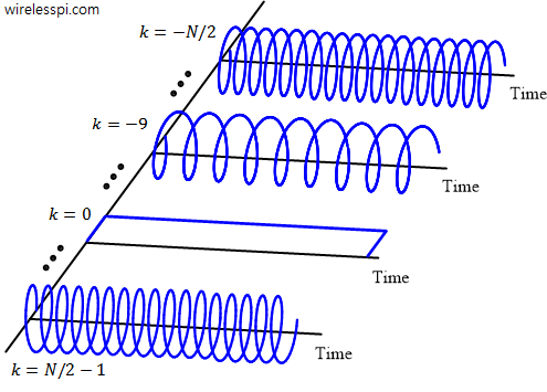
• Analogous to continuous-time limits of $-\tau/2$ to $\tau/2$, the discrete-time index $n$ goes from $-N/2$ to $N/2-1$. On a similar note, we choose $N$ frequency indices represented by $k$ with the same range, i.e., from $-N/2$ to $N/2-1$. These $N$ sinusoids are plotted in the figure below.

  

For a sufficiently high sample rate $f_s=1/T_s$ with no aliasing, time domain samples of $x(t)$ are taken at intervals of $nT_s$. Therefore, from Eq (\ref{equation-dft-1}), the sampled version of $x(t)$ becomes
\[
x[n] = \sum_{k=-N/2}^{N/2-1} X_k e^{j\omega_k t}\Bigg|_{t=nT_s} = \sum_{k=-N/2}^{N/2-1} X_ke^{j2\pi kf_0 (nT_s)}
\]

because $\omega_k = 2\pi f_k = 2\pi kf_0$. Since there are $N$ samples within one period $\tau=1/f_0$ of the fundamental frequency, we have $\tau=NT_s$ or $f_0T_s=1/N$. Thus, the above expression yields
\[
x[n] = \sum_{k=-N/2}^{N/2-1} X_k e^{j2\pi \frac{k}{N}n}
\]

With an analogous argument that led to Eq (\ref{equation-fourier-transform}), we get the final expression.

This is the well-known Discrete Fourier Transform (DFT). All this relation is telling us is that a discrete-time signal can be thought of as made up of $N$ complex sinusoids with frequencies $2\pi k/N$. And the contribution $X_k$ of each such sinusoid can be determined by elementwise product of the signal with the corresponding complex sinusoid but with an opposite sign.

I/Q Signals in Frequency Domain: Signal DNA

The complex amplitude $X_k$ displays the contribution of a complex sinusoid having frequency $2\pi k/N$ in forming the resultant signal $x[n]$. A larger value represents a higher amplitude of that particular frequency sinusoid in forming the original signal and vice versa. Even a real signal in time domain has $I$ and $Q$ parts in frequency domain!

Just like reductionism in the form of atoms, cells, bits and pixels described at the start of this article, complex sinusoids play the same role in signal analysis and synthesis. From this viewpoint, Fourier Transform is not a good terminology; it should have been called Signal Cells or Signal DNA.

This view of I/Q signals in frequency domain is plotted in the figure below. A true understanding of Fourier Transform is shown as the complex numbers $X_k$ in blue determining the amplitude and phase of their respective complex sinusoids.

These $X_k$, shown in blue above, form the frequency domain $I$ and $Q$ components which is a very different thing than time domain $I$ and $Q$ encountered in Part 1. The time domain signal is constructed from the summation of all these pink complex sinusoids.

Relation between Phase Angle and Phase Shift

To gain some insight into the relation between phase angle in I/Q plane of one domain and the phase shift of a sinusoid in I/Q plane of the other domain, let us recall the frequency domain idea above: A unit impulse in one domain (e.g., frequency) corresponds to a complex sinusoid in the other domain (e.g., time). Mathematically,
\[
\text{Fourier Transform of}~~\delta(\omega-\omega_0) \quad \rightarrow \quad e^{j\omega_0 t}
\]

The figure above reproduces this concept so that it can be compared with the figure coming next. The impulse in frequency domain exists entirely on the $I$ axis. There is no phase angle here due to which the complex sinusoid in time domain has it peak at zero. Both cosine and sine are not phase shifted with respect to their zero reference.

Due to Fourier Transform linearity, multiplying both sides of the above equation by a constant keeps the relation intact. This constant can be a real number such as $4$ or a complex number such as $e^{j\theta}$. Thus, we can change the above expression to
\[
\text{Fourier Transform of}~~e^{j\theta}\delta(\omega-\omega_0) \quad \rightarrow \quad e^{j\theta}e^{j\omega_0 t} = e^{j(\omega_0 t + \theta)}
\]

This result is plotted in the figure below.

Observe how the phase angle lifts the impulse and now this signal has both $I$ and $Q$ parts in frequency domain. In time domain, this phase angle $\theta$ appears as a phase shift of this complex sinusoid which is why it does not have its peak at time zero. This can also be seen in sine and cosine waveforms that are now phase shifted with respect to their zero reference.

Therefore, the phase angle of the unit impulse in frequency $IQ$-plane determines the starting location of the sinusoids in time $IQ$-plane. This is illustrated in the figure below.

• The top plot shows the same four sinusoids that add together to form a square wave we saw earlier. Notice zero starting location for all sines which represents a zero phase in frequency I/Q plane.
• The bottom plot shows those four sinusoids with a nonzero phase in frequency I/Q plane. Notice how each of them is now phase shifted with respect to the ideal zero reference. Do you think that they add up to form a square wave too? The answer is no.

Conclusion

• In general, a time domain I/Q signal can be taken as a sequence of two parallel signals treated as a set of complex numbers with $I$ (real) and $Q$ (imaginary) parts. The phase angle of each sample represents its orientation on the complex plane which is determined by the relative signs and magnitudes of the two parts. There is important information hidden in this phase angle, whether caused by nature or introduced by engineers.
• In frequency domain, a signal has a spectrum that also consists of both $I$ (real) and $Q$ (imaginary) parts. Owing to the property of Fourier Transform, the phase angle in this frequency I/Q plane determines the phase shift of each time domain constituent sinusoid as compared to zero time reference.