Convolution and Fourier Transform

One question I am frequently asked is regarding the definition of Fourier Transform. A continuous-time Fourier Transform for time domain signal $x(t)$ is defined as
\[
X(\Omega) = \int _{-\infty} ^{\infty} x(t) e^{-j\Omega t} dt
\]

where $\Omega$ is the continuous frequency. A corresponding definition for discrete-time Fourier Transform for a discrete-time signal $x[n]$ is given by
\[
X(e^{j\omega}) = \sum _{n=-\infty} ^{\infty} x[n] e^{-j\omega n}
\]

where $\omega$ is the discrete frequency related to continuous frequency $\Omega$ through the relation $\omega = \Omega T_S$ if the sample time is denoted by $T_S$. Focusing on the discrete-time Fourier Transform for the discussion, here is the question often asked regarding these relations.

Textbooks and online resources answer this question in significant details through a signals viewpoint. I have also written about the concept of frequency domain where we learned that most practical signals can be constructed from a large number of complex sinusoids with different amplitudes and phases. Later, we explored the idea behind Discrete Fourier Transform (DFT) where it was shown that the Fourier Transform is actually a correlation process with a set of such sinusoids to find out how much contribution each of them has towards constructing the signal under study. Both of these articles looked at this problem from a signals perspective too.

Today, we are going to see this concept from a systems perspective. Towards the end, we will also come to know why convolution in time domain is multiplication in frequency domain. Let us start with defining a system.

A System

In wireless communications and other applications of Digital Signal Processing (DSP), we often want to modify a generated or acquired signal. A device or algorithm that performs some prescribed operations on an input signal to generate an output signal is called a system. Amplifiers in communication receivers and filters in image processing applications are some systems that we interact with in daily lives.

Impulse Response

An impulse response is just the output response of a system to a unit impulse $\delta[n]$ as an input. It is a way of characterizing how a system behaves. Impulse response is also a signal sequence and it is usually denoted as $h[n]$.

As an example, when a tuning fork is hit with a rubber hammer, the response it generates is a back and forth vibration of the tines that disturb surrounding air molecules for a certain amount of time: that is its impulse response. In a very similar manner, when a system is `kicked’ by a unit impulse signal, the whole sequence of samples it generates can be viewed as its impulse response, an example of which is illustrated in the figure below.

A Simple Filter

The simplest system in the field of DSP is a moving average filter. To see the idea behind it, consider taking a running average of 5 samples in an input signal to generate one output sample. The output $y[n]$ to an input $x[n]$ is then
\begin{align*}
y[n] &= \frac{1}{5}\Big( x[n] + x[n-1] + x[n-2] + x[n-3] + x[n-4]\Big) \\
&= \frac{1}{5}x[n] + \frac{1}{5}x[n-1] + \frac{1}{5}x[n-2] + \frac{1}{5}x[n-3] + \frac{1}{5}x[n-4]
\end{align*}

The above expression can be written for $M=5$ as
\[
y[n] = \sum \limits_{k=0}^{M-1} \frac{1}{M} \cdot x[n-k]
\]

If the factors $1/M$ are taken as the coefficients of the impulse response $h[n]$ of a filter, then it can be generalized to any impulse response as
\begin{equation}\label{equation-convolution}
= \sum \limits_{k=0}^{M-1} h[k] x[n-k]
\end{equation}

Since this impulse response is of finite length, it is one example of a Finite Impulse Response (FIR) filter. Naturally, we can then modify these taps of $h[n]$ to design a filter that is better suited to the application at hand. If you already know about it, you could recognize Eq (\ref{equation-convolution}) as a convolution equation. This is a general expression for finding the output $y[n]$ of a system with impulse response $h[n]$ when the given input is $x[n]$.

These points seem insignificant but this individual scaling and time shifting are actually tightly coupled with our definition of Fourier Transform through complex exponentials.

What Makes an Input Appropriate?

With the convolution equation at hand, our purpose is to find an input $x[n]$ that results in the simplest possible output $y[n]$ (if you’re thinking about a unit impulse, remember that it is used to define the impulse response itself). Observing that the input part of the expression involves $n-k$ in Eq (\ref{equation-convolution}), most inputs will generate a complicated output. For instance, for a quadratic input $n^2$, we have
\[
x[n] = n^2 \qquad \qquad \Longrightarrow \qquad \qquad x[n-k] = (n-k)^2=n^2 +k^2 -2nk
\]

and hence
\[
y[n] = \sum \limits_{k=0}^{M-1} h[k] x[n-k] = \sum \limits_{k=0}^{M-1} h[k] \Big(n^2 +k^2 -2nk\Big)
\]

which does not lend itself to further simplification. On the other hand, only an input containing $n$ in its power can give rise to a factorization in two different terms.

The Impact of $n$ in the Power

Taking $x[n]=a^n$ as a general example, we have
\begin{align}
y[n] &= \sum \limits _{k=0}^{M-1}h[k]a^{n-k} = a^n \sum \limits _{k=0}^{M-1}h[k]a^{-k} \label{equation-input-output} \\
&= x[n]\sum \limits _{k=0}^{M-1}h[k]a^{-k} \nonumber
\end{align}

The most interesting part of the above result is that an input $x[n]=a^n$ simply appears at the output as it is, multiplied with an expression that is a function of

• the system impulse response $h[n]$ itself, and
• the constant $a$ in the input.

Our next step is to find out an appropriate value of this constant $a$.

Finding the Constant $a$

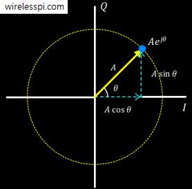
Focus on the expression $\sum _{k=0}^{M-1}h[k]a^{-k}$ and let us call it $H$. Consider a general complex value for $a$ which covers the real values as a special case. This complex number can be given as $a=Ae^{j\theta}$ where $A$ is the magnitude and $\theta$ is the angle. This is known as the polar representation of a complex number. If you do not particularly like expressions involving $e^j$, there is a rectangular representation too given by
\begin{align*}
a_I &= A \cos \theta \\
a_Q &= A \sin \theta
\end{align*}

Both of these representations are shown in the figure below.

For the magnitude $|a|=A$, there are three different possibilities.

Enter the Complex Sinusoids

What exactly is this third option $A=1$ above, i.e., $x[n]=a^n=e^{j\theta n}$? Recall from the last figure above that $e^{j \theta}$ is a point in complex plane with x and y coordinates given by $\cos \theta$ and $\sin \theta$, respectively. With the inclusion of time index $n$, this complex number starts moving in an anticlockwise manner because $e^{j \theta n}$ implies
\begin{align*}
x_I[n] &= \cos \theta n \\
x_Q[n] &= \sin \theta n
\end{align*}

With each time index $n=0, 1, 2, \cdots,$ this complex number rotates one further step anticlockwise and this rotation keeps increasing the angle with $n$. Thus, the angle $\theta$ turns out to be its frequency of rotation and denoted from hereon as $\omega$. Many authors actually use $\theta$ instead of $\omega$ to emphasize this point. Such a rotating waveform is a complex sinusoid, a continuous version of which is plotted below with each discrete time index marked with a cross. The I and Q (i.e., x and y) components of this waveform from the above expression can also be seen as a cosine and sine, respectively.

With an understanding of these complex sinusoids, we find their impact on a system next.

Forming the Frequency Response

Let us plug the above signal $x[n]=e^{j\omega n}$ in Eq (\ref{equation-input-output}).
\begin{align}
y[n] &= \sum \limits _{k=0}^{M-1}h[k] e^{j\omega (n-k)} = e^{j\omega n} \sum \limits _{k=0}^{M-1} h[k] e^{-j\omega k} \nonumber\\
&= x[n]\cdot H\left(e^{j \omega}\right) \label{equation-output}
\end{align}

In technical terms, these complex sinusoids are the eigenfunctions of Linear Time-Invariant (LTI) systems. It is straightforward to notice that not only the input $x[n]$ appears at the output as is, but also the system output becomes independent of the input magnitude. The resulting expression is known as the frequency response of the system, as opposed to the impulse response in time domain.

To explore what this frequency response is about, consider what the above relation
\[
y[n] = x[n]\cdot H\left(e^{j \omega}\right) = e^{j\omega n} \cdot H\left(e^{j \omega}\right)
\]

is telling us. In words, it says that any system can be probed through a set of complex sinusoids with different frequencies $\omega$ and the output response $H\left(e^{j \omega}\right)$ can thus be measured. This system will treat these $\omega$ in one of the following possible ways.

• Pass untouched
• Amplify
• Suppress to some extent
• Completely block

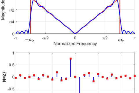
An example of such a system treating the complex sinusoids in this manner is shown below. This is a graphical manifestation of the frequency response $H\left(e^{j \omega}\right)$ discovered in Eq (\ref{equation-frequency-response}) above.

This is exactly what we happens when an impulse is input to a system in time domain. Remember from another article on DFT examples that DFT of an all-ones sequence is a single impulse in frequency domain. Owing to the duality of time and frequency domains, the inverse is also true: the DFT of a single impulse in time domain is an all-ones rectangular sequence in frequency domain, which is nothing but several complex sinusoids of equal magnitudes.. In other words, a single impulse in time domain being input into a system causes a sequence of $N$ complex sinusoids with equal magnitudes in frequency domain!

Through enough data points $\omega$, we can faithfully represent the frequency response of that system. Next time you see a spectral plot like the one shown below, you would immediately recognize that it represents the discriminatory behavior of the system for each frequency $\omega$ that has been obtained by probing it with a large number of frequencies.

Matched Filtering

Why is there a negative sign in the definition of frequency response of Eq (\ref{equation-frequency-response}) while the complex sinusoids are defined with a positive sign (anticlockwise rotation)? This is because we multiply and sum (i.e., correlate) the signal $h[n]$ with each negative frequency (clockwise rotation, $e^{-j\omega n}$) complex sinusoid so that only the same frequency term (but opposite rotation, $e^{+j\omega n}$) exactly cancels the power in the exponent at each step $n$ and finally produce a large single value at the summation output. It is another manifestation of matched filtering we so often employ in many other science (and psychology) problems.

How Does All This Relate to Convolution

When I was a student, the most striking idea for me was that convolution in time domain is multiplication in frequency domain. Why not multiplication in time domain and multiplication in frequency domain? As I grew more experienced, I discovered that multiplication in time domain is actually multiplication in frequency domain! I have described this concept in the article on convolution from an intuitive viewpoint. Coming back to convolution as multiplication in frequency domain, this single property has done more than anything else in the adoption of digital signal processing in so many fields.

It can be seen from Eq (\ref{equation-output}) that the very definition of convolution relies on the complex sinusoidal inputs. I said before that signal processing applications are not only interested in the current sample $x[n]$ but they also access and weigh the previous input samples $x[n-k]$. This time shifting operation to access the past samples $x[n-k]$ gives rise to $n-k$ term in the definition of convolution. The main point here is that factorization of $n-k$ terms in the power as multiplication of two powers — one in $n$ and the other in $-k$ — enable us to write this operation as multiplication in frequency domain of two different functions.

The derivation of the Goertzel algorithm is a good example of the relation between convolution and the frequency domain.