How a Frequency Locked Loop (FLL) Works

We saw before how a carrier frequency offset distorts the received signal. Later, we also described the classification of frequency synchronization techniques according to the availability of the symbol timing. Today, we will learn about the workings of a frequency locked loop.

Background

A Phase Locked Loop (PLL) is a device used to synchronize a periodic waveform with a reference periodic waveform. It is an automatic control system in which the phase of the output signal is locked to the phase of the input reference signal. In the article referred above, we also discussed that for a very small frequency offset, a PLL is sufficient for driving the phase error between the Rx signal and the local oscillator output to zero. However, a PLL fails to operate for a large CFO and hence an acquisition aid must be invoked prior to handing the signal over to the PLL. Some of the common acquisition aids adopted for this purpose are the following.

• Frequency sweeping: In this technique, the frequency of the local oscillator is swept over an uncertainty interval during acquisition until a phase lock is achieved. Then, the frequency sweeping is stopped to avoid an unnecessary increase in the phase variance.
• Multi-stage acquisition: It consists of using a large filter bandwidth during the acquisition process and then switching to a narrow loop filter after the lock. Or a large CFO is significantly reduced by using a non-timing-aided technique in the feedforward mode. A timing-aided scheme is applied later to compensate for any residual CFO.
• Frequency Locked Loop (FLL): In an FLL, a Frequency Error Detector (FED) generates an error signal corresponding to the difference in frequency between a reference and an output waveform to drive the loop similar to a PLL. An FLL can be used in parallel with a PLL such that the former operates during acquisition and loss of lock while the latter during steady state tracking.

FLL Components

A block diagram of an FLL is drawn in the figure below. Just like a carrier PLL and a timing PLL, a frequency locked loop consists of the following components.

• Frequency Error Detector (FED): As mentioned above, a frequency error detector determines the frequency difference between a reference input waveform and a locally generated waveform. According to the amount of that difference, it generates an error signal denoted as $e_D[n]$.
• Loop Filter: A loop filter sets the dynamic performance limits of an FLL as well. Moreover, it helps filter out noise and irrelevant frequency components generated in the frequency error detector. Its output signal is denoted as $e_F[n]$.
• Numerically Controlled Oscillator (NCO): An NCO generates a local discrete-time and discrete-valued waveform with a phase as close to the phase of the reference signal as possible. For a continuously changing phase, i.e., a frequency difference, an NCO consistently changes its phase, thus tracking the frequency of the reference.

In such a feedback setting with established components of an FLL in place (loop filter and NCO), our focus is now on devising a suitable frequency error detector that can generate an error signal $e_D[n]$ proportional to the frequency difference to enable the tracking of the reference frequency.

The FLL we are going to discuss here as a case study is a timing-aided feedback system. Therefore, the frequency error detector operates at the symbol rate, i.e., the error signal $e_D[m]$ it generates is in terms of symbol time $m$. Other kinds of frequency error detectors are also common which operate at a rate higher than the symbol rate, one of which is an FLL based on band edge filters.

An Example FLL

Our current FLL setup assumes the following set of conditions.

• The CFO is small enough that timing can be acquired before its compensation (however, this CFO is still large enough that a PLL alone cannot do the job).
• With correct timing, Nyquist no-ISI condition is also satisfied and each symbol spaced sample is (almost) independent from the contribution of the neighbouring symbols.
• No training sequence is available and the Rx makes decisions on the optimal symbol spaced samples. Given the role of CFO, these decisions need not be correct.

Consider the block diagram in the figure below that describes the implementation of the overall FLL in terms of complex signals. The same FLL can be drawn for real signals. The matched filter output is downsampled by $L$ to produce a signal at the symbol rate. During each symbol time $m$, this signal is multiplied with the complex conjugate decisions $\hat a^*[m]$ from the symbol detector and fed to the Frequency Error Detector (FED). The FED produces an error signal $e_D[m]$ that is upsampled by $L$ to match the sample rate of the loop filter and the NCO. Subsequently, it is smoothed out by the loop filter and drives an NCO that accordingly adjusts the phase of its output waveform at the sample rate $T_S$.

Now we develop an understanding of how this structure eliminates the CFO. We can see in the article on the effect of a carrier frequency offset that the signal arriving at the Rx $x(nT_S)$ is ideally a shaped symbol stream that is distorted by a CFO. Coming to the FLL here, this is multiplied with another complex sinusoid generated by the NCO in the figure above. The net effect is that the symbols are rotated by a frequency error $F_{0:e}$ arising from the difference between these two frequencies. Following exactly the same steps as in that article, the phase of the matched filter output is then given by
\begin{equation*}
\measuredangle z(mT_M) = \measuredangle a[m] + 2\pi F_{0:e} m
\end{equation*}

The interpretation of the above equation is as follows. Assuming a QPSK constellation with a unit amplitude, the data symbols $a[m]$ are just phase shifts of $\pm \pi/2$ and $\pm 3\pi/2$. These symbol values are now rotating anticlockwise with a frequency $F_{0:e}$!

Phase Shift Keying (PSK) Modulation

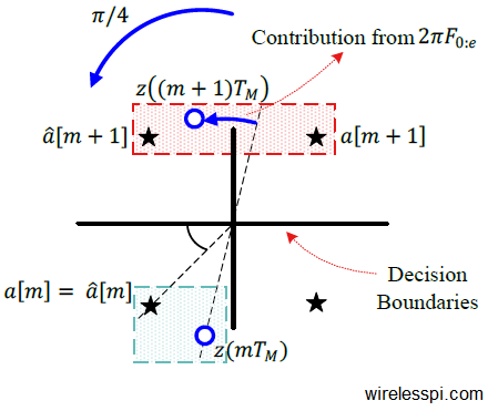
In the case of any digital modulation scheme, these $T_M$-spaced samples are input to the symbol detector that generates symbol decisions $\hat a[m]$. The detector makes the decisions based on the minimum distance rule. At time $m$, it selects the constellation symbol $\hat a[m]$ closest to the matched filter output $z(mT_M)$. This is drawn in the figure below where $z(mT_M)$ must be mapped to the symbol decision $\hat a[m]$.

Here is the interesting part: Looking at the shaded green box at the bottom of this figure, $\measuredangle z(mT_M)$ $-$ $\measuredangle \hat a[m]$ is a little less than $+\pi/4$. Thus, we can write
\begin{equation*}
\measuredangle z(mT_M) = \measuredangle a[m] + 2\pi F_{0:e} m, \quad \text{and} \quad \hat a[m] = a[m]
\end{equation*}

Now at time $m+1$,
\begin{align*}
\measuredangle z\big\{(m+1)T_M\big\} &= \measuredangle a[m+1] + 2\pi F_{0:e} (m+1), \\
&= \measuredangle a[m+1] + 2\pi F_{0:e} m+2\pi F_{0:e} , \quad \text{and} \quad \hat a[m+1] \neq a[m+1]
\end{align*}

It is evident that the factor $2\pi F_{0:e}$ has rolled over the matched filter output $z\big\{(m+1)T_M\big\}$ across the symbol boundary, as illustrated by the shaded red box at the top of the above figure. However,
\begin{equation*}
\left|\measuredangle z\big((m+1)T_M\big) – \measuredangle \hat a[m+1]\right| < \pi/4 \end{equation*} This characteristic can be utilized to devise a frequency error detector as follows.

• To remove the data modulation phase, multiply the matched filter output $z(mT_M)$ with conjugate of the detector decision $\hat a^*[m]$.
  \begin{equation*}
  y(mT_M) = \hat a^*[m]\cdot z(mT_M)
  \end{equation*}

  which implies
  \begin{equation*}
  \measuredangle y(mT_M) = -\measuredangle \hat a[m] + \measuredangle z(mT_M)
  \end{equation*}

  Since the detector makes decisions based on the nearest constellation point, the above term always lies within the range $(-\pi/4,+\pi/4)$. To prove this point, imagine $\measuredangle y(mT_M)$ being greater than $+\pi/4$. This implies that the difference between $\measuredangle z(mT_M)$ and $\measuredangle \hat a[m]$ is greater than $\pi/4$ which in a QPSK constellation means that the detector has not selected the nearest constellation point, which is not true.

• Next, we draw $\measuredangle y(mT_M)$ in the figure below for $F_{0:e} = + 0.05$ on the left and for $F_{0:e} = -0.05$ on the right. As expected, $\measuredangle y(mT_M)$ is an increasing ramp for $F_{0:e}>0$ and a decreasing ramp for $F_{0:e} <0$. We need a frequency error detector that at least leads the NCO to the right direction of frequency error movement.

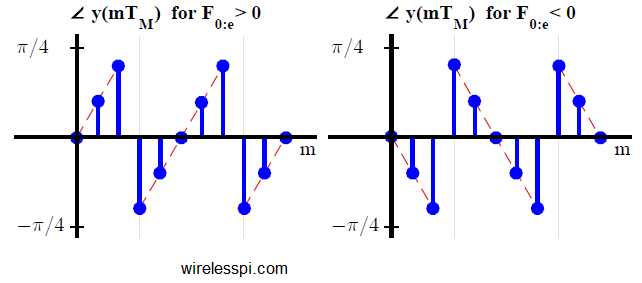
  Here, the main point to note is that the form of the frequency error detector is still not finalized, since an average of the above mentioned signal will tend towards zero for both a positive and a negative $F_{0:e}$! A little amount of processing is required to configure a proper FED such that on average, its output has the same sign as $F_{0:e}$.

• To produce an error signal with the same sign as $F_{0:e}$, all we need to do is to ensure that in $\measuredangle y(mT_M)$ plots above, there should be more positive samples than the negative samples for a positive $F_{0:e}$ and vice versa. For this purpose, a new frequency error detector can be devised as
  \begin{equation}\label{eqFreqSyncConstellationFED}
  e_D[m] =
  \begin{cases}
  \measuredangle y(mT_M) & \quad -\lambda < \measuredangle y(mT_M) < \lambda \\ e_D[m-1] & \qquad\qquad\text{otherwise} \end{cases} \end{equation}

  where $\lambda$ is a threshold value, the absolute value of which is less than $\pi/4$. Let us see how this forms a valid frequency error siganl.

To understand the operation of this frequency error detector, consider the figure above where $e_D[m]$ is plotted along with $\measuredangle y(mT_M)$ (in dashed green line) for $\lambda = \pi/6$. Observe that the average of $e_D[m]$ is positive for a positive $F_{0:e}$ and negative for a negative $F_{0:e}$. The reason can be grasped by looking at $e_D[m]$ for a positive $F_{0:e}$ to the left of the above figure.

1. At time $m=0$, both $\measuredangle y(mT_M)$ and the error $e_D[m]$ are zero.
2. At time $m=1$, $\measuredangle y(mT_M)$ is less than the threshold $\lambda$. Therefore, the error $e_D[m]$ is also the same.
3. At time $m=2$, $\measuredangle y(mT_M)$ goes past the threshold $\lambda$. Consequently, the error $e_D[m]$ is equal to its previous value (which is less than $\measuredangle y(mT_M)$).
4. At time $m=3$, $\measuredangle y(mT_M)$ rolls over towards $-\pi/4$. Because its magnitude is still greater than the threshold $\lambda$, the error $e_D[m]$ again remains unchanged to a positive value. Thus it becomes greater than $\measuredangle y(mT_M)$ which is negative.

The key to working of this error detector is that the loss incurred at step 3 above is smaller as compared to the gain at step 4. The average value of the error signal $e_D[m]$ is hence positive. A corresponding argument holds for a negative $F_{0:e}$.

The operation of this frequency error detector is explained for a QPSK modulation above. The same idea can easily be extended to an $M$-PSK constellation by observing that $\measuredangle (mT_M)$ lies between $-\pi/M$ and $+\pi/M$. The error signal $e_D[m]$ thus can be generated by choosing a threshold $\lambda$ less than $\pi/M$.

Quadrature Amplitude Modulation (QAM)

For PSK constellations, the decision regions are very simple which is not the case for QAM constellations. Therefore, a little ingenuity is required to extend the idea of phase based FED to QAM modulation schemes. For a $16$-QAM constellation, for example, one possible solution is as follows.

Observe from the figure below that a $16$-QAM constellation consists of $2$ QPSK constellations, one in the interior and one at the exterior, plus an $8$-PSK constellation in the center. The strategy chosen is as follows.

When the detector makes a decision in favour of any one of the two QPSK constellations, the FED output $e_D[m]$ is computed as before in Eq \eqref{eqFreqSyncConstellationFED}. However, when the decision falls in the region defined by $8$-PSK constellation, it can be left unchanged. Thus, the expression for such a frequency error detector is written as

To see the effect of such an error detector on the carrier frequency synchronization for a $16$-QAM modulation, the matched filter output $z(mT_M)$ and the FLL output are drawn in the figure below for a Square-Root Raised Cosine pulse with excess bandwidth $\alpha=0.5$. The parameter $\lambda$ is chosen to be $\pi/6$ while a damping factor $\zeta=1/\sqrt{2}$ and a loop noise bandwidth of $B_{FLL} T_M=3\%$ drive the FLL response at an $E_b/N_0$ $=$ $15$ dB. Notice the three PSK constellations that form the $16$-QAM are clearly visible which perhaps led towards the discovery of this carrier recovery scheme. Finally, after the convergence in the right figure, the constellation is still affected by a small phase offset and a PLL is needed to drive this error towards zero.

A similar strategy with appropriate modification can be adopted for other higher-order QAM modulation schemes.