An Introduction to Constant Modulus Algorithm (CMA)

In many kinds of equalizers such as maximum likelihood sequence estimation, the channel response is available at the Rx through any channel estimation procedure that requires a training sequence. For adaptive equalization such as Least Mean Square (LMS) equalizers or Decision Feedback Equalization (DFE), first the training sequence symbols and then symbol decisions are employed to tune the equalizer taps. There are many applications, however, where the Rx needs to acquire the equalizer coefficients without any help from the Tx in the form of known symbols. This is a non-data-aided scenario that is primarily required in mobile communication systems where the Rx can lose the signal due to channel fading or blockage and blind acquisition is needed after the signal returns. Some of the other applications are a general purpose radio to demodulate most wireless communication signals, military radios, signal monitoring and point to multi-point networks.

Blind equalization, also known as self-recovering equalization, is the process of choosing the equalizer taps without any help from a training sequence or symbol decisions. Constant Modulus Algorithm (CMA) is the most prevalent blind equalization technique that was devised by Godard in 1980.

Intuition

The CMA is very similar to the LMS algorithm with the only difference being in the performance function. In case of the LMS algorithm, the performance function was the squared error reproduced below.
\begin{equation*}
\text{Mean}~ |e[m]|^2 = \text{Mean}~ \left|a[m] – y[m]\right|^2 = \text{Mean}~ \left|a[m] – z[m]*q_l[m]\right|^2
\end{equation*}

where $a[m]$ are the data symbols, $z[m]$ is the equalizer input, $y[m]$ is the equalizer output, and $q_l[m]$ is the $l^{th}$ equalizer tap at time $m$. The question is what to do in the absence of any data symbols $a[m]$ or their decisions $\hat a[m]$.

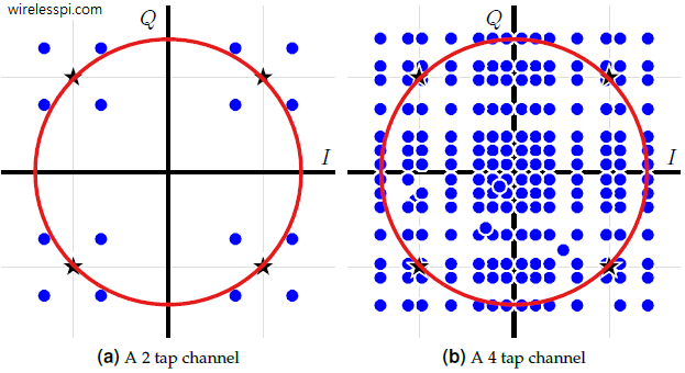
For this purpose, we first consider the scatter plot of QPSK symbols received through a multipath channel. When multiple taps are convolved with the Tx symbols, one beautiful example for a simple channel was shown here after downsampling the signal to $L=1$ sample/symbol. That figure is redrawn below in the top subfigure for a 2-tap channel and in the bottom subfigure for a 4-tap channel. Regardless of how convoluted (pun intended) the signal looks like as the multipath scatters the Tx symbols all over the 2D plane, we can still observe a structure in these figures. From our knowledge of wireless channels, we have seen that the channel acts on the Rx signal in a systematic manner unlike noise. This gives us a hope of recovering the signal even without any data or channel knowledge.

Now suppose that symbol timing recovery, even imperfect, is in place and the matched filter output $z[m]$ at $L=1$ sample/symbol is available. More importantly, we are not interested in carrier phase recovery at this stage. Then, with all the scattered symbols in this 2D plane, one strategy is to form a ring in this 2D plane that passes through the desired symbol locations as drawn in the figures above. For a normalized QPSK constellation,
\begin{equation*}
\left\{a_I[m],a_Q[m]\right\} =
\begin{cases}
+\frac{1}{\sqrt{2}}, +\frac{1}{\sqrt{2}} \\
+\frac{1}{\sqrt{2}}, -\frac{1}{\sqrt{2}} \\
-\frac{1}{\sqrt{2}}, +\frac{1}{\sqrt{2}} \\
-\frac{1}{\sqrt{2}}, -\frac{1}{\sqrt{2}}
\end{cases}
\end{equation*}

The ring that passes through these symbols has a radius equal to 1. From the figure above, if the distance between the location of actual Rx samples and this ring is minimized, the channel is implicitly equalized regardless of the complexity of the channel. In this respect, this is a very interesting strategy that is different than other equalization techniques where training or decisions are available.

The Algorithm

In light of the above, the performance criterion used by the CMA is
\begin{equation*}
\text{Mean}~ \bigg(\Big|y[m]\Big|^2 – 1\bigg)^2
\end{equation*}

where $|y[m]|^2$ is the energy of the symbol-spaced samples scattered around the constellation and 1 is their desired energy concentrated in a constellation circle. The next steps of the derivation are very similar to the LMS algorithm. Mean $(|y[m]|^2 – 1)^2$ can be dealt with as a function of $2L_q+1$ equalizer taps $q_l[m]$ and a unique minimum point on the error surface can be reached by removing the mean, then starting at any point and taking a small step opposite to the gradient with respect to the equalizer tap weights.
\begin{equation}\label{eqEqualizationCMA1}
q_l[m+1] = q_l[m] – \frac{d}{dq_l[m]} \bigg(\Big|y[m]\Big|^2 – 1\bigg)^2
\end{equation}

As before, $q_l[m]$ means the $l^{th}$ equalizer tap at symbol time $m$. The derivative in the above expression is written for each $l$ $=$ $-L_q$, $\cdots$, $L_q$, as
\begin{equation}\label{eqEqualizationCMA2}
\frac{d}{dq_l[m]} \bigg(\Big|y[m]\Big|^2 – 1\bigg)^2 = 2\bigg(\Big|y[m]\Big|^2 – 1\bigg) \cdot \frac{d}{dq_l[m]}~ \Big|y[m]\Big|^2
\end{equation}

Using $y[m] = z[m] * q_l[m]$, we can open $|y[m]|^2$ by considering the case for a real signal only that can be later generalized to complex signals. Then, for each $l$ $=$ $-L_q$, $\cdots$, $L_q$, we can write
\begin{align*}
\frac{d}{dq_l[m]} \Big|y[m]\Big|^2 &= 2 y[m]\cdot \frac{d}{dq_l[m]} \sum _{l=-L_q}^{L_q}q_l[m] z[m-l] \\
&= 2y[m]\cdot z[m-l]
\end{align*}

Plugging back in Eq (\ref{eqEqualizationCMA2}) and ignoring the irrelevant constants,
\begin{equation*}
\frac{d}{dq_l[m]} \bigg(\Big|y[m]\Big|^2 – 1\bigg)^2 ~ = ~ y[m]\cdot z[m-l] \cdot \bigg(\Big|y[m]\Big|^2 – 1\bigg)
\end{equation*}

Finally, substitute this value back in the tap update Eq (\ref{eqEqualizationCMA1}) and introduce the step size $\mu$ for a smooth convergence to obtain the final expression for a CMA equalizer.

where the conjugate appears as a result of the same derivation for complex signals.

Comments

A few comments about the constant modulus algorithm are now in order.

Generalization

The actual CMA equalizer is a generalized version of the algorithm derived above. There, instead of taking the magnitude squared of the equalizer output $y[m]$, any other value of $p$ can be employed. So the performance criterion becomes
\begin{equation*}
\text{Mean}~ \bigg(\Big|y[m]\Big|^p – 1\bigg)^2
\end{equation*}

Following a similar derivation, the generalized CMA update equation becomes
\begin{equation*}
\begin{aligned}
q_l[m+1] = q_l[m] &- \mu\cdot y^*[m]\cdot \Big|y[m]\Big|^{p-2} \cdot z[m-l] \cdot \bigg(\Big|y[m]\Big|^p – 1\bigg)\\
&\text{for each }l = -L_q,\cdots,L_q
\end{aligned}
\end{equation*}

Phase Locked Loop (PLL)

Observe from the expression of the CMA equalizer that it exploits the magnitude of the Rx samples to compensate for the channel. Consequently, the convergence can happen at any phase and a Phase Locked Loop (PLL) can be run at the output with the CMA equalizer to correct for the rotated symbols in a non-data-aided fashion.

Mode Switch

As happens with the algorithms working without any knowledge of a training sequence or symbol decisions, the convergence time of the CMA equalizer is significantly longer than the LMS algorithm. This is the cost of having no known symbols within the Tx sequence. Furthermore, the symbol decisions are not available until the convergence of the equalizer. When that eventually happens, the tap update mechanism can be switched from CMA to LMS algorithm in a decision-directed fashion.

Multi-Modulus Algorithm (MMA)

From the intuition behind CMA algorithm shown in the figure above, it is evidently more suited to a PSK constellation. To better cope with QAM signals, a Multi-Modulus Algorithm (MMA) separately penalizes the dispersion of the inphase and quadrature parts of the equalizer output. This is equivalent to fitting the constellation on to a square instead of a circle. A natural advantage of MMA is that it converges towards the steady state equalizer taps with a correct phase offset and hence a carrier recovery loop is not required at the final stage.