Wireless communication is energy inefficient due to the nature of the medium that spreads out energy in an unguided manner, as opposed to guided media like optical fiber and coaxial cable. To avoid wastage of power, one solution is to lower the transmit (Tx) power but then the receiver is left with the herculean task of efficiently demodulating the receive symbols at a low SNR. This article describes the design and implementation of one such receiver.
Background
The physical layer of a receiver system consists of three major parts, namely the frontend, the inner receiver, and the outer receiver. The frontend is the domain of RF circuit designers while coding theorists handle the outer receiver. A DSP engineer is mainly concerned with inner receiver design.
This includes estimation and compensation for gain control, synchronization (timing, carrier frequency and phase), channel estimation and equalization. The target is to present almost perfect symbols perturbed by additive white Gaussian noise only to the decoder.
At low SNRs, acquisition is difficult as the signal is not clearly differentiated from the noise. In this regime, data-aided algorithms that exploit a training sequence are more accurate but prove costly for bandwidth, decision-directed algorithms that utilize previous decisions suffer from error propagation and a non-data-aided approach simply fails to work. The only way to overcome the noise is significant averaging that only happens in the decoder part. This leads to the idea that soft decisions from decoders can be utilized to refine the unknown synchronization and channel parameters.
The Iterative Principle
The basic principle of an iterative receiver is to squeeze the maximum amount of information from the received samples before making a final decision on data symbols. This implies that the soft output of the channel decoder can be employed to reconstruct the symbols on which synchronization and channel estimation algorithms can be applied again in an iterative manner. Since the iterative decoders improve the output SNR, this feedback loop results in a refined signal acquisition as well.
In this article, I focus on a multicarrier system like Orthogonal Frequency Division Multiplexing (OFDM) for the design of a low SNR receiver. This is because many modern wireless communication systems such as 4G, 5G and WiFi use multi-carrier techniques at their physical layers. Code-aided synchronization is helpful in OFDM systems because inaccurate timing, frequency and channel estimates give rise to Inter-Symbol Interference (ISI) and Inter-Carrier Interference (ICI).
Transmitter
The block diagram of a coded OFDM transmitter is drawn below.

The transmit process can be broken down into the following steps.
- A turbo-encoder, operating at a rate of $r$, processes an information segment of length $B$ bits. This encoder employs two recursive systematic convolutional (RSC) encoders.
- The resulting coded bit stream undergoes bit interleaving through a pseudo-random interleaver, ensuring that the coded bits exhibit approximate independence from each other, which is crucial for the subsequent decoding stages at the receiver.
- Following bit interleaving, the coded bit stream is mapped onto Quadrature Amplitude Modulation (QAM) symbols.
- This symbol stream is then organized into segments, each consisting of $N_c$ subcarriers.
- Here, the symbols are assumed to be in frequency domain. Hence, an $N_c$-point Inverse Fast Fourier Transform (IFFT) is applied to convert the symbol stream into a time domain signal (a certain number of subcarriers, denoted as $N_g$, are reserved as guards on both edges of the band to meet filtering requirements).
- Next, a cyclic prefix of length $N_{cp}$ is inserted at the beginning of each OFDM segment. The choice of $N_{cp}$ is made such that it exceeds the delay spread of the channel to mitigate Inter-Symbol Interference (ISI).
- Subsequently, the resulting symbols are multiplexed with a training sequence $T_k$ of length $N_p$, essential for the acquisition stage at the receiver. This training sequence is designed similar to those used in IEEE 802.11a systems, featuring two identical halves.
- To form a complete OFDM frame, $N$ such segments are assembled to form the signal $x(n)$. These samples are then transmitted to the SDR hardware. I usually use USRP B210 and Analog Devices ADALM Pluto for my experimentation purpose.
The Wireless Channel
A frequency-selective wireless channel that transforms a modulated signal is described by the following equation.
\[
h(t) = \sum _{l} \alpha_l \delta (t – \tau_l) \nonumber
\]
Here, $\alpha_l$ represents the complex amplitude distributed as a Gaussian random variable while $\tau_l$ is the delay of the $l$-th tap, with the maximum delay being less than the length of cyclic prefix $N_{cp}$ in samples. The system assumes a quasi-static block-fading channel that remains constant within each frame but varies independently for subsequent frames.
Since the channel output is a convolution between the transmit signal and channel impulse response, the sampled received signal from the SDR hardware is expressed as
\begin{equation}\label{eqSystemTime}
y(n) = e^{j2 \pi \epsilon n/N_c} \sum _{l=0} ^{L-1} h(l) x(n-l) + w(n)
\end{equation}
Here, $\epsilon$ represents the carrier frequency offset (CFO) between the Tx and the Rx normalized by the OFDM symbol rate, $h(n)$ is the sampled channel response with $L$ taps, $x(n)$ is the transmitted signal and $w(n)$ is the Gaussian noise.
Receiver Design
The overall operation of the receiver is illustrated in the figure below.

Initially, the starting sample of the received sequence is identified using a frame synchronization algorithm (or coarse timing in OFDM), facilitating the determination of the coarse frequency offset. Subsequently, fine timing and fine frequency are estimated, followed by SNR estimation. After removing the cyclic prefix, the Discrete Fourier Transform (DFT) output is given by
\[
Y_k = H_k X_k + W_k
\]
where $k = 0,1,\cdot\cdot\cdot,N_c-1$ is the subcarrier index, $X_k$ is the transmitted QAM symbol and $H_k$ is the DFT of the impulse response $h[n]$.
\[
H_k = \sum _{l=0} ^{L-1} h(l) e^{-j 2 \pi l\frac{k}{N_c}}
\]
This is known as the channel frequency response at subcarrier $k$. Finally, $W_k$ is the additive white Gaussian noise. All these quantities are in frequency domain.
However, in case of imperfect synchronization, this expression contains distortions [1] as
\begin{equation}\label{eqSystemFreq}
Y_k = \frac{\sin (\pi \epsilon)}{N_c ~\sin (\pi \epsilon/N_c)} e^{j \pi \epsilon (N_c-1)/N_c}~ H_k X_k + \text{ICI}(k) + W_k
\end{equation}
Next, channel estimation is carried out in the frequency domain, enabling equalization of the received signal on a subcarrier basis. Before the first iteration, any residual phase offset resulting from the remaining frequency offset is eliminated, a crucial step for relatively long block lengths of iterative decoders. Finally, the iterations involving the soft decoder, channel estimation, and equalizer are executed, as depicted in the above figure.
Coarse Synchronization
In OFDM, the training sequence is periodic and frame detection algorithm utilizes two autocorrelators that correlate the training sequence with a delayed version of itself. Based on Eq (\ref{eqSystemTime}), an autocorrelator metric $J(m)$ can be defined as
$$
\begin{equation}
\begin{aligned}
J(m) &=& \sum _{n=0} ^{N_c-1} y(n-m) ~ y^\ast(n-m-N_w) \nonumber\\
&=& e^{j2\pi \epsilon N_w/N_c} \times \left(\texttt{Magnitude Term} \right)
\end{aligned}
\end{equation}\label{equation-jm}
$$
where $N_w$ is the window length of operation. This window should be equal to at least the minimum repetition length of the training sequence. In the above expression, there is a phase term and a magnitude term.
- Since the complex samples in two halves of periodic training sequence are the same, the normalized CFO gives rise to a phase term.
- The magnitude term is a function of sequence alignment, ICI and their cross-terms.
Next, the particular shape of the plateau can be used to identify the starting point of a frame in terms of a differentiator defined by
\begin{equation*}
J'(m) = |J(m)|^2 – |J(m-N_c/2)|^2
\end{equation*}
The differentiator produces a metric that gradually rises until the frame start and then descends with the same slope. Since the Automatic Gain Control (AGC) significantly disrupts peak detection algorithms, this algorithm employs both an instantaneous peak detector and a group peak detector in addition to the differentiator.
Typically, an initial coarse frequency estimate could be derived at this stage by observing the phase of the coarse timing reference. However, operating at a relatively lower SNR renders the coarse frequency estimate unreliable to the extent that it may not need to be estimated at all. Instead, we rely on the cross-correlation for a more precise timing estimate and the corresponding finer CFO estimate, as we see next.
Fine Synchronization
In fine timing synchronization, a cross-correlation is calculated between the stored noiseless training sequence and the received sequence, adjusted by the coarse frequency estimate. This process begins a few samples before the frame boundary estimate and concludes a few samples after it. The fine timing estimate may experience an offset by a few samples due to the channel convolution. Consequently, the actual frame start is positioned a few samples before the estimated marker, incorporating a safety margin to the left of the OFDM symbol boundary attributable to the cyclic prefix. This offset subsequently manifests as a phase shift after the Discrete Fourier Transform (DFT) and integrates into the unknown channel characteristics.
After finding the boundaries, the noisy received training is separated from the data frame. A CFO estimate can now be estimated by using the two repetitive portions of this sequence. From Eq (\ref{equation-jm}), the CFO is given by
\[
\hat \epsilon = \frac{N_c}{2\pi N_w} \arctan \{J(\hat m)\}
\]
The estimate $\hat m$ is the starting sample of the sequence in the above expression.
SNR Estimation
For SNR estimation, first the signal power is calculated from I and Q samples of the received training as
\[
\hat P_S = \frac{1}{N_c/2} \sum _{n=0} ^{N_c/2-1} \Big[ y_I(n)y_I(n+N_c/2) + y_Q(n) y_Q(n+N_c/2) \Big]
\]
On a similar note, the noise power turns out to be
\[
\hat P_W = \frac{1}{2N_c/2} \sum _{n=0} ^{N_c/2-1} \left[ \left\{y_I(n) – y_I(n+N_c/2)\right\}^2 + \left\{y_Q(n) – y_Q(n+N_c/2) \right\}^2 \right]
\]
The SNR estimate is then given by $\hat P_S/\hat P_W$. Separate estimates of signal and noise power are also required as an input to the turbo decoder.
Channel Estimation
In the initial iteration, the standard channel estimates are derived from the two recurring segments of the received training.
\[
\hat H_k = \frac{0.5(Y_k + Y_{k+N_c/2})}{T_k}
\]
The subsequent data symbols in the frequency domain are equalized by dividing them with their corresponding channel estimates, and the resultant signal is then fed into the turbo decoder.
Residual CFO Tracking
At this point, a residual frequency offset persists due to a slight difference between the actual and estimated fine frequency offset. The significance of this remaining CFO lies in two key reasons within our context.
- Firstly, signals at low SNR do not yield improved frequency estimates on average, as they are susceptible to well-known threshold effects.
- Secondly, even when the estimated CFO closely approximates the actual value, the extended block lengths inherent in iterative decoders introduce sufficient phase shift across the frame, rendering additional turbo processing futile.
To conserve power and bandwidth, I implemented a solution that capitalizes on the rotation of constellation symbols. In systems employing multi-carrier or single-carrier configurations with frequency-domain equalization, the actual signal is inherently divided into multiple segments. In the case of traditional single-carrier systems, the received signal can be segmented into various sections for this purpose. As outlined in [1], a frequency offset introduces not only an Inter-Carrier Interference (ICI) term in the received symbols due to sampling at incorrect frequency instances but also imparts a rotation to the frequency domain symbols via a time-variant phasor $e^{j 2 \pi \epsilon [n (N_c+N_{cp}) + N_{cp}]/N_c}$, where $n$ denotes the OFDM symbol index. Consequently, the phase increment from one OFDM symbol to the next is determined by the angle.
\[
\theta_F = 2 \pi \epsilon \frac{(N_c+N_{cp}) + N_{cp}}{N_c}
\]
At high SNR, the subcarrier symbol rotations induced by residual local offsets are typically minor and can be effectively tracked by the channel estimator. However, in low SNR scenarios, the situation changes. Instead of recalculating the frequency offset that has already undergone refinement, we leverage this characteristic by employing a non-data-aided Viterbi and Viterbi phase estimator on a segment-by-segment basis.
\begin{eqnarray*}
\gamma_k &=& |Y_k|^2 e^{j 4 \measuredangle Y_k}\\
\hat \theta_F &=& -\frac{1}{4} \measuredangle \sum \gamma_k
\end{eqnarray*}
Given that the estimated phase offset is non-data-aided for QAM modulation, it is constrained within the interval $−\pi/4 \le \hat \theta_F \le \pi/4$. To eliminate the modulo $\pi/2$ operation for tracking the phase shift, it is essential to unwrap the estimates by
\[
\tilde{\theta}(n+1) = \tilde \theta(n) + \text{mod}\left(\hat \theta_F(n) – \tilde \theta(n)-\pi/4,\pi/2\right) – \pi/4
\]
This approach for mitigating the impact of residual CFO not only eliminates the necessity of incorporating frequency correction within the iterative loop but also provides resilience against a substantial residual CFO. This is because, for residual CFO correction to be integrated into the iterative loop, it must be sufficiently small to ensure decoder convergence to approximately true soft symbols. Ultimately, this solution demands no additional training or pilot overhead and can be implemented as a non-data-aided approach, even in scenarios characterized by low SNR.
Iterative Processing
To maintain a simple receiver structure, I incorporate only channel estimation and equalization within the iterative loop, as mentioned earlier in the receiver block diagram. If $a_i$ and $b_i$ denote the two bits Gray-mapped onto the $i^{th}$ QPSK symbol, the soft estimates of received symbols are computed as
\begin{equation}\label{eqSoftSymbols}
\hat X_k^{(q)} = \sum _{a_i,b_i} P_{a_i}^{(q)} P_{b_i}^{(q)} Z_{a_i,b_i}
\end{equation}
Here, $P_{a_i}$ and $P_{b_i}$ represent the a posteriori probabilities of bits $a_i$ and $b_i$ for the $i^{th}$ symbol, and $Z_{a_i, b_i}$ is the corresponding constellation symbol, i.e., $Z_{a_i, b_i} = \pm 1 \pm j$ for QPSK. The subscript $q$ denotes the iteration number. The presence of the interleaver allows us to express this symbol probability as the product of individual bit probabilities.
The a posteriori probabilities $P_{a_i}$ and $P_{b_i}$ can be determined if the Log-Likelihood Ratios (LLRs) of each individual bit are known. This is because
\begin{eqnarray*}
\text{LLR}(a_i) &= \log \left\{ \frac{Pr\left( a_i = +1\right)}{Pr\left( a_i = -1\right)} \right\} = \log \left\{ \frac{Pr\left( a_i = +1\right)}{1-Pr\left( a_i = +1\right)} \right\} \\
&= \log {\frac{\sum _{S_{a_i} \in S_1} e^{-|Y_k – H_k S_{a_i}|^2/\hat {P}_W}}{\sum _{S_{a_i} \in S_0} e^{-|Y_k – H_k S_{a_i}|^2/\hat {P}_W }}}
\end{eqnarray*}
Here, $\log$ is taken with respect to base $e$, $\hat {P}_W$ represents the estimated noise power, and $S_0$ and $S_1$ denote the sets of symbols in the original QPSK constellation corresponding to the bit $a_i$ being 0 and 1, respectively. Continuing from the above equation,
\[
Pr\left( a_i = +1\right) = \frac{e^{\text{LLR}(a_i)}}{e^{1+\text{LLR}(a_i)}}, \qquad Pr\left( a_i = -1\right) = \frac{1}{e^{1+\text{LLR}(a_i)}}
\]
By incorporating the aforementioned expressions and symbol values for $Z_{a_i,b_i}$ into Eq \eqref{eqSoftSymbols} and performing some manipulations, we obtain
\[
\hat X_k ^{(q)} = \tanh\frac{\text{LLR}\left(a_i^{(q)}\right)}{2} + j ~\tanh\frac{\text{LLR}\left(b_i^{(q)}\right)}{2}
\]
\begin{eqnarray}\label{eqSoftSymbols16QAM}
\hat X_k ^{(q)} &= \tanh\frac{\text{LLR}\left(a_{i,1}^{(q)}\right)}{2} \left\{2 + \tanh\frac{\text{LLR}\left(a_{i,2}^{(q)}\right)}{2} \right\} + \nonumber \\
& j\cdot \tanh\frac{\text{LLR}\left(b_{i,1}^{(q)}\right)}{2}\left\{2 + \tanh\frac{\text{LLR}\left(b_{i,2}^{(q)}\right)}{2} \right\}
\end{eqnarray}
Using the updated soft symbol, the channel estimate at the $k^{th}$ subcarrier can be updated as
\begin{equation}\label{eqChannelUpdate}
\hat H_k ^{(q)} = \frac{Y_k}{\hat X_k^{(q)}}
\end{equation}
As zero-forcing and MMSE equalization excessively amplify the noise, with the former having a more pronounced effect than the latter, improved performance can be achieved for a constant modulus constellation like QPSK by maintaining the amplitudes unaltered and solely correcting for the phase offset in each iteration.
\[
\hat Y_k^{(q+1)} = Y_k \cdot e^{-j\measuredangle \hat H_k^{(q)}}
\]
To mitigate computational complexity, the channel updates and subsequent equalization can be halted either after a fixed number of iterations or upon reaching a predetermined convergence criterion.
Performance Evaluation
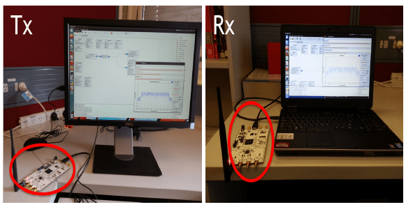
In a standard application, baseband signal processing algorithms are executed in software on a host computer. Meanwhile, the analog and digital frontends are implemented on an SDR hardware, connecting to the host computer through a high-speed link.

In the experimental setup illustrated in the above figure, a desktop and a laptop were employed to connect to their respective SDRs to conduct the experiments. The transmission utilized the ISM band at 2.4 GHz with a bandwidth of $8$ MHz.
The main parameters are configured as per the table below.

The Tx hardware conducts Digital Up-Conversion (DUC) to the specified sample rate, while the amplification and conversion to the carrier frequency are handled by the Tx analog frontend. On the receiver side, this process is reversed, with the RF frontend amplifying and downconverting the received signal. The signal is then sampled and decimated by the Digital Down-Conversion (DDC). The received samples are transferred from the Rx hardware to the PC through GNU Radio, where they are stored in a file. Due to the computational complexity of the turbo decoding algorithms, which prevents real-time implementation on a general-purpose processor, baseband signal processing is subsequently carried out offline.
In this system, there are two types of receiver implementations:
- Iterative receiver: This implementation follows the iterative processing framework discussed earlier, incorporating feedback to the channel estimation and equalization units. Parameter updates in the iterative receiver occur for the first $5$ iterations, and the total number of turbo decoder iterations is set to $8$.
- Conventional receiver: This implementation employs the same acquisition algorithms as the iterative receiver but does not involve any feedback to the channel estimation and equalization units. Turbo decoding is performed without iteration feedback. All other parameters, including the number of turbo decoder iterations are kept the same for both receivers.
The SDRs are placed in an open-door extension of the hall to investigate the results. The Block Error Rate (BLER) is drawn in the figure below. This observed gap of 1.5-2 dB between the conventional and iterative receivers aligns with research results available. Minor discrepancies may arise due to factors such as the channel profile, constraint length at the encoder, generator polynomials, and the number of iterations at the decoder, among others.

References
[1] M. Speth, A. Fechtel, G. Fock, and H. Meyr, Optimum receiver design for wireless broad-band systems using OFDM, Part I, \em{IEEE Transactions on Communications}, Vol. 47, No. 11, 1999.