The frontend of the transceiver plays a crucial role in determining the ultimate system performance. In a previous article, we described how a superheterodyne architecture helps in enhancing the selectivity and sensitivity of the receiver. Some of the main issues with a superheterydone receiver are the image frequency and a large form factor due to multiple conversion stages. Today we discuss a direct conversion architecture, also known as zero-IF and homodyne.
Recall from the concept of frequency domain that a real sinusoid at the Local Oscillator (LO) output has two impulses in its spectrum, one at a positive frequency $+F_{\text{LO}}$ and the other at the negative frequency $-F_{\text{LO}}$. A clue for the root cause of the image frequency problem appears when the LO frequency $F_{\text{LO}}$ is equal to the carrier frequency $F_C$. In this scenario, the image band is the same as the band of the desired signal and hence cannot be eliminated by any image reject filter, see the figure below and put $F_{\text{LO}}= F_C$.

Next, we explain how direct conversion solves the image frequency problem.
What is a Zero-IF (Direction Conversion or Homodyne) Architecture
One solution to this issue is to employ complex signal processing and mix the signal with a complex sinusoid of frequency $-F_{\text{LO}}$ which has a single impulse in its spectrum at that frequency. This operation produces a complex signal whose spectrum is simply a shifted version of the real signal spectrum due to convolution with this single impulse. This is drawn in the figure below for $F_{\text{LO}}=F_C$ where one-sided spectral translation of the real Rx signal from $F_C$ to $F_C-F_{\text{LO}}=0$ eliminates the need of an image reject filter. It must be remembered that the complete elimination happens in a theoretical sense only since imperfections in the analog frontend contribute towards a limited suppression.

With $F_{\text{LO}}=F_C$ option available as above, we can downconvert the Rx signal directly to the baseband. There are different terminologies used for this architecture as follows.
- Direct conversion: There are no intermediate stages and the translation is performed in one step.
- Zero-IF: The baseband spectrum can also be considered as an IF at $F=0$.
- Homodyne: This terminology reflects a conversion philosophy different than a heterodyne architecture.
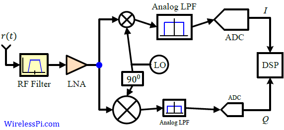
A block diagram for a zero-IF architecture is drawn in the figure below.

After the preselection filter and low noise amplifier, downconversion to baseband is accomplished through a pair of mixers and the quadrature sinusoids forming the complex sinusoid. The complex signal thus produced is filtered by two lowpass filters, one in the $I$ arm and the other in the $Q$ arm, that remove the double frequency term, select the desired band and suppress the adjacent channels. As a result, the lowpass filters need to exhibit sharp cutoff characteristics. Although the bulk of signal processing seems to happen in analog domain, the opposite is true. A direct conversion Rx simply downconverts the passband signal to the baseband and leaves the job of cleaning up all the real-world impairments to the DSP engine, some of which we describe next.
Challenges for Zero IF
While the concept of directly downconverting a signal seems the most logical option, there are a number of challenges that need to be overcome for realization of a zero-IF architecture.
DC offset
This is the most severe problem at the baseband output signal of a direct conversion Rx. A conversion to the band around zero frequency makes the desired signal vulnerable to offset voltages that can saturate the subsequent stages. To understand this issue, consider that there are two inputs to the mixer, one coming from the LO and the other from the LNA. This results in a phenomenon known as LO leakage shown in the figure below that arises due to the following factors (the corresponding indices are marked on the figure).

- The isolation between the mixer ports connected to the LO and the LNA output is not infinite which causes the LO sinusoid to leak through to the other input of the mixer.
- A similar argument holds for the LNA input as well.
- To worsen the situation, a strong in-band interferer within the passband of the RF preselection filter also leaks from the LNA output to the mixer port connected to the LO and hence gets multiplied with itself creating another DC offset. This is also shown in the figure above.
Due to both of these leakages, the LO sinusoid is mixed with a delayed version of itself — known as self-mixing — thus producing a DC (Direct Current) component at the mixer output entering the lowpass filter. Assuming the LO signal as $A \cos 2\pi(k/N)n$ and the leaked version coming into the other mixer input as $B\cos (2\pi(k/N)n-\phi)$, we have
\begin{equation*}
2 A\cos \left(2\pi \frac{k}{N}n \right)\cdot B\cos \left(2\pi \frac{k}{N}n – \phi\right) = \underbrace{AB\cos \phi}_{\text{DC offset}} + AB \cos\left(2\pi \frac{2k}{N}n – \phi\right)
\end{equation*}
While the double frequency term is eliminated through the lowpass filter, the DC offset is summed with the desired signal within the baseband and saturates the subsequent electronic stages. From an SDR perspective, this is particularly harmful for the Analog to Digital Converter (ADC) that prepares the digital signal for DSP applications during demodulation. Moreover, this DC offset can vary with time when the LO signal leaks through the antenna, gets radiated outwards and reflected back to the Rx from nearby objects. For rapidly changing reflections, it can become difficult to isolate this time-varying offset.
In addition to creating the DC offset issue, the LO sinusoid leaked through the antenna acts as an unmodulated carrier wave that deteriorates the performance of the nearby receivers operating in the same band by creating additional interference. It should be remembered that some of these issues are also present in a heterodyne Rx but to a much lesser extent. Since the desired signal falls at the intermediate frequency $F_{\text{IF}}$, the mixing may only arise from strong interferers within the band and the DC offset thus produced can be easily filtered out.
IQ Imbalance
In a zero-IF Rx, complex signal processing is employed through analog circuitry to directly shift the target spectrum to baseband as shown before. For this purpose, both $I$ and $Q$ mixers, LPFs and ADCs must impart identical gain and $90^{\circ}$ phase difference across the whole signal bandwidth in their respective $I$ and $Q$ arms, an impossible task to achieve in analog components.
A figurative example of $IQ$ imbalance is shown in the figure below as different sizes of the mixers, LPFs and the ADCs as well as the tilts. Consequently, amplitude and phase mismatches occur between each pair of parallel sections in $I$ and $Q$ paths. Furthermore, quadrature mixing through a pair of real sinusoids (i.e., a complex sinusoid) is required for downconversion generated by a single LO. This is done by using the relation $\cos (A-90^{\circ})$ $=$ $\sin A$ and hence the cosine output of an LO is phase shifted by $90^{\circ}$ to produce the sine output. As expected, this phase shift is not exactly $90^{\circ}$ due to the manufacturing tolerances.

To see the effect of this $IQ$ imbalance coming through the LO only, denote the amplitude or gain error of the LO as $\gamma_\Delta$ and phase error of the LO as $\theta_\Delta$ and assume that half of the gain and phase errors lie on the $I$ arm of the LO while the other half on the $Q$ arm.
$$\begin{equation}
\begin{aligned}
V_{\text{LO},I}(t) \: &= \sqrt{2}\left(1+\frac{\gamma_\Delta}{2}\right)\cos \left( 2\pi F_C t + \frac{\theta_\Delta}{2}\right) \\
V_{\text{LO},Q}(t) &= -\sqrt{2}\left(1-\frac{\gamma_\Delta}{2}\right)\sin \left( 2\pi F_C t – \frac{\theta_\Delta}{2}\right)
\end{aligned}
\end{equation}\label{eqNoTitleVLO}$$
where, as before, the factor $\sqrt{2}$ is used for normalization purpose. Now consider a $4$-QAM waveform at passband arriving at the Rx antenna.
\begin{equation*}
r(t) = v_I(t) \sqrt{2} \cos 2\pi F_C t – v_Q(t) \sqrt{2}\sin 2\pi F_C t
\end{equation*}
Next, we multiply the real signal $r(t)$ above with the LO complex output in Eq (\ref{eqNoTitleVLO}). Here, we use the regular trigonometric sum product formulas in addition to lowpass filtering the high frequency components.
\[
\begin{aligned}
x_I(t) \: &= v_I(t) \left(1+\frac{\gamma_\Delta}{2}\right)\cos \left( \frac{\theta_\Delta}{2}\right) – v_Q(t) \left(1+\frac{\gamma_\Delta}{2}\right)\sin \left( \frac{\theta_\Delta}{2}\right)\\
x_Q(t) &= v_Q(t) \left(1-\frac{\gamma_\Delta}{2}\right)\cos \left( \frac{\theta_\Delta}{2}\right) + v_I(t) \left(1-\frac{\gamma_\Delta}{2}\right)\sin \left( \frac{\theta_\Delta}{2}\right)
\end{aligned}
\]
Since $(1+\gamma_\Delta)/2$ and $(1-\gamma_\Delta)/2$ are constants (but not equal), notice that the above equations are very similar to those encountered during the study on the effect of a phase offset on QAM constellation. Therefore, we can follow a similar derivation on our way to symbol rate sampling and matched filtering which yields the final result as
\[
\begin{aligned}
x_I(mT_M)\: &= \left(1+\frac{\gamma_\Delta}{2}\right) \left\{a_I[m] \cos \left( \frac{\theta_\Delta}{2}\right) – a_Q[m]\sin \left( \frac{\theta_\Delta}{2}\right)\right\}\\
x_Q(mT_M) &= \left(1-\frac{\gamma_\Delta}{2}\right)\left\{ a_Q[m] \cos \left( \frac{\theta_\Delta}{2}\right) + a_I[m] \sin \left( \frac{\theta_\Delta}{2}\right)\right\}
\end{aligned}
\]
- Notice from the above equation that when the gain error $\gamma_\Delta$ is zero, it reduces to the same equation regarding the phase offset in a QAM constellation.
- On the other hand, when the phase error $\theta_\Delta$ is zero, the data symbols $a_I[m]$ and $a_Q[m]$ get scaled by different factors.
We have seen the effect of a phase offset $\theta_\Delta$ in isolation on a QAM constellation. Now let us draw the gain error $\gamma_\Delta$ to view its effect in isolation from the phase offset. For this purpose, the left subfigure below illustrates a $4$-QAM signal constellation for a gain error of $\gamma_\Delta=-0.8$ while the right subfigure shows the combined effect of gain error $\gamma_\Delta=-0.25$ and phase error $\theta_\Delta=-30^\circ$.

In addition to an inaccurate mapping on the Rx constellation, such an imbalance affects the performance of the synchronization loops in the demodulator.
Advantages of Zero-IF Architecture
The challenges mentioned above were significant enough that the zero-IF architecture mostly remained in the shadows in comparison to the superheterodyne Rx. In the past years, there have been a number of developments that contributed towards its widespread adoption and now can be found in most consumer radios.
Chip integration
With a growing list of applications, a wireless device needs to support multiple bands and more bandwidth. A direct conversion to baseband eliminates the need for an IF filter and IF amplifiers. A pair of lowpass filters at baseband are more easily integrated as active lowpass filters instead of lossy and off-chip fixed-IF devices. These active filters cover a wide range of bandwidth since they can be tuned from hundreds of kHz to hundreds of MHz. A wide range of RF frequencies can also be covered by simply adjusting the LO frequency. This flexibility coming from integrated programmable baseband filters greatly reduces the PCB footprint of a zero-IF radio.
Cost
Through elimination of some components and integration of others, the zero-IF design reduces the system cost as compared to other architectures. This is in addition to cost savings that come from the flexibility of adding new bands without rigorous planning.
Power
Since a zero-IF architecture directly reduces the frequencies of interest to baseband, the analog circuits are designed at the lowest frequency possible thus reducing power consumption.
Concluding Remarks
A direct conversion receiver reduces system complexity, bypasses the image frequency issue, contains enhanced chip integration and exhibits higher selectivity.
The problems associated with such radios are usually controlled through analog optimization and digital correction. For both the DC offset and IQ imbalance, tracking algorithms are employed to compensate for their respective distortions. A device like AD9371 is a typical example of a zero-IF transceiver covering a wide range of frequencies from $300$ MHz to $6$ GHz. Each Tx can cover between $20$ MHz and $100$ MHz of bandwidth while each Rx bandwidth span is from $5$ MHz to $100$ MHz.
One important point to remember here is that relatively imprecise tolerances still lead to successful signal recovery for lower-order modulation schemes such as BPSK and $4$-QAM. On the other hand, for higher-order modulation schemes such as $64$-QAM and $256$-QAM, even little inaccuracies in DC offset and $IQ$ imbalance add up and corrupt the baseband signal beyond repair. As the manufacturing tolerances cross certain thresholds, no amount of baseband DSP can then recover the data symbols. Nevertheless, as the technology improves in favour of a small form factor with digital calibrations, direct conversion receivers have become a sound choice in many digital radio systems.