Kalman filter is one of the most important but not so well explained filter in the field of statistical signal processing.
As far as its importance is concerned, it has seen a phenomenal rise since its discovery in 1960. One of the major factors behind this is its role of fusing estimates in time and space in an information-rich world. For example, position awareness is not limited to radars and self driving vehicles anymore but instead has become an integral component in proper operation of industrial control, robotics, precision agriculture, drones and augmented reality. Kalman filter plays a major role in the signal processing segment of these applications.
As far as the poor explanation is concerned, this is due to one of the following reasons.
- Some simple tutorials on the web are loaded with many unnecessary numerical examples, which make the main ideas seem more complicated than they actually are.
- Many other tutorials on this topic are written for people with advanced degrees. The derivation goes through a winding road of linear algebra, probability and statistics and ends in a summary of the algorithm as shown in the figure below.
- Both of the above two approaches use confusing terminology (e.g., what is $n-1|n-1$), and do not sufficiently explain the real intuition behind the Kalman filter.

My goals of writing this article are as follows.
- I believe that every equation in mathematics is telling a story. Here, I explain the reader from the ground up what story the above 5 equations are telling us.
- It also describes enough intuition to give the practitioners a new perspective on Kalman filter.
For this purpose, I start with how we form our opinions in everyday life.
How We Form Opinions
We all believe that we form solid opinions based on facts and logical reasoning. While this is rarely true, let us review our opinion forming process when a new evidence comes up. As a child, our mind is a blank slate and our beliefs are developed according to what parents and teachers tell us during the initial few years.
As we grow up, we encounter a new evidence regarding a particular matter. How should we update our opinion now? We can derive the result through Bayesian estimation but that would become too technical, so let us employ simple common sense.
The process of updating that opinion is usually a linear combination of prior belief and new evidence (or measurement) that can be mathematically written as
\begin{equation}\label{equation-updated-opinion}
\text{Updated Opinion} = \text{Weight}_\text{prior}\times\text{Prior Belief} ~~+~ \text{Weight}_\text{measure}\times\text{New Evidence}
\end{equation}
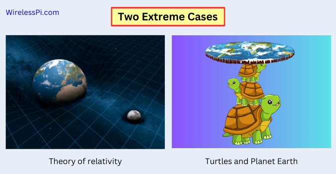
The terms $\text{Weight}_\text{prior}$ and $\text{Weight}_\text{measure}$ are included here because the updated opinion largely depends on the trust a person has in their prior belief as well as the new evidence. This point can be understood with the help of following two extreme cases.
- Remember the first time you heard about Einstein’s theory of relativity. Space and time can be bent, it sounds completely unbelievable (for me, no fiction has ever come closer). The evidence, however, is overwhelming whether it is in the form of planetary motion tracking, red and blue shifts in the light of distant stars from relativistic Doppler or clock adjustments in GPS satellites. As a consequence, one can set $\text{Weight}_\text{measure}$ of new evidence or measurement at a maximum value (high trust) and $\text{Weight}_\text{prior}$ of prior belief at a minimum value (low trust) in Eq (\ref{equation-updated-opinion}). A rational person’s updated opinion is that the theory of relativity is true.
\[
\text{Updated Opinion} \quad \leftarrow \quad \text{Weight}_\text{measure}\times \text{New Evidence}
\]The stronger the evidence, the greater the updated belief, thanks to $\text{Weight}_\text{measure}$. The same goes for any other scientific discovery.
- Consider the place of planet Earth in our universe. In his doctoral dissertation, the linguist John R. Ross writes about an encounter between the philosopher and psychologist William James and an old lady.
Planet Earth
The following anecdote is told of William James. […] After a lecture on cosmology and the structure of the solar system, James was accosted by a little old lady.
"Your theory that the sun is the centre of the solar system, and the earth is a ball which rotates around it has a very convincing ring to it, Mr. James, but it’s wrong. I’ve got a better theory," said the little old lady.
"And what is that, madam?" inquired James politely.
"That we live on a crust of earth which is on the back of a giant turtle."
Not wishing to demolish this absurd little theory by bringing to bear the masses of scientific evidence he had at his command, James decided to gently dissuade his opponent by making her see some of the inadequacies of her position.
"If your theory is correct, madam," he asked, "what does this turtle stand on?"
"You’re a very clever man, Mr. James, and that’s a very good question," replied the little old lady, "but I have an answer to it. And it’s this: The first turtle stands on the back of a second, far larger, turtle, who stands directly under him."
"But what does this second turtle stand on?" persisted James patiently.
To this, the little old lady crowed triumphantly,
"It’s no use, Mr. James—it’s turtles all the way down."
Here, a believer assigns $\text{Weight}_\text{prior}$ of this prior belief about planet Earth at a maximum value (high trust) while $\text{Weight}_\text{measure}$ of new evidence at a minimum value (low trust) in Eq (\ref{equation-updated-opinion}). As a consequence, no amount of scientific evidence can change their mind and their updated opinion is the same as their prior belief.
\[
\text{Updated Opinion} \quad \leftarrow \quad \text{Weight}_\text{prior}\times \text{Prior Belief}
\]In political and religious matters, psychologists have discovered that if $\text{Weight}_\text{prior}$ is initially large, presenting new evidence actually strengthens the prior belief!

Most of our opinions in everyday life lie on the spectrum between these two extremes, more on this shortly. Next, we describe how to gauge an opinion.
Gauging an Opinion
We start with how trust can be expressed in a numerical form.
Trust as a Number
It is said that mathematics is the language of the universe. In the past decades, the rise of computers compels us to map most phenomena into numbers, whether it’s the the heat flow in the heart of a star or chemical activity in our brains. Nevertheless, when we talked about matters related to human nature like thoughts and emotions, we did not really think in numbers.
At least as far as trust is concerned, this has changed with the advent of product review systems (think Amazon and Trustpilot) where a level of trust can be established on a scale of 1 to 5. People now hardly purchase anything with a low rating.
Assume that we have access to a numerical form of trust in our prior belief and new evidence and let us call it Precision (we will discuss next where this number comes from). This implies that Eq (\ref{equation-updated-opinion}) can be modified as
\begin{equation}\label{equation-precision}
\text{Updated Opinion} = \color{blue}{\text{Precision}_\text{prior}}\times\text{Prior Belief} ~~+~ \color{blue}{\text{Precision}_\text{measure}}\times\text{Measurement}
\end{equation}
where we have replaced new evidence with measurement because a scientific evidence is usually a result of some experimental measurement with a certain precision (for mathematicians, precision is the same as accuracy for a zero-mean random variable that is assumed true here).
Now we turn towards quantifying this precision.
How to Quantify Precision
In general, the quantities involved in the estimation process are not deterministic but random variables, i.e., a variable whose possible values are numerical outcomes of a random experiment. The likelihood of each of those values occurring is given by a probability distribution function, an example of which is drawn in the figure below.

Most well known properties of a random variable are its mean and variance. While the mean is easily understood as the average value of all outcomes, the variance ($\sigma^2$) is a measure of how spread out that set of numerical outcomes is around that average value. In mathematical speak, for example, $68\%$ of observations in a Gaussian distribution fall within the first standard deviation ($\sigma$). Mean and variance are also marked in the figure above.
It is evident that the smaller the variance, the more compact the probability distribution is and vice versa.
- Since all the possible outcomes then lie close to the average value, a smaller variance gives rise to a higher precision.
- On the other hand, a higher variance implies that sample values of the random variable under consideration are spread all over the place; a sign of less precision.
As a consequence, the inverse variance $1/\sigma^2$ of a random measurement can be taken as a good indicator of its precision.
\[
\text{Precision} = \frac{1}{\sigma^2}
\]
Let $1/\sigma_\text{prior}^2$ denote the precision of our prior belief and $1/\sigma_\text{measure}^2$ as that of the new evidence or measurement. Thus, Eq (\ref{equation-precision}) can now be expressed as
\begin{equation}\label{equation-sigma}
\text{Updated Opinion} = \frac{1}{\sigma_\text{prior}^2}\times\text{Prior Belief} ~~+~ \frac{1}{\sigma_\text{measure}^2}\times\text{Measurement}
\end{equation}
The problem here is that precision is unbounded and it can by any large or small number that loses its value in obtaining a fair result.
Normalized Precision
As an example, my friend Dan Boschen currently has a reputation of almost 52k at DSP Stack Exchange, the second highest rating in all the users of that forum. On the other hand, the highest-rated user at Mathematics Stack Exchange has a reputation of 618k. Does this mean that his opinion is 12 times more precise than Dan’s? The answer is no, since people simply ask more math questions than DSP questions. So what we actually need is a normalization step.
If one has an equal trust in both prior belief and new evidence, then fusing them should produce the same value, not the double. For example, if you know a priori that your weight is 150 lbs and the new machine you bought measures it as 150 lbs, your updated result is 150 lbs, not 300 lbs. Therefore, the normalized precisions here should be $0.5$ and their sum should be $1$.
Let us denote the normalized precision of the prior belief as $\kappa_\text{prior}$ (the Greek letter kappa) and that of evidence or measurement by $\kappa_\text{measure}$. Normalization implies that the weights are now defined as
$$\begin{equation}
\begin{aligned}
\kappa_\text{prior} = \frac{\text{Precision}_\text{prior}}{\text{Precision}_\text{prior}+\text{Precision}_\text{measure}} &= \frac{\frac{1}{\sigma_\text{prior}^2}}{\frac{1}{\sigma_\text{prior}^2}+\frac{1}{\sigma_\text{measure}^2}}=\frac{\sigma_\text{measure}^2}{\sigma_\text{prior}^2+\sigma_\text{measure}^2}\\
\kappa_\text{measure} = \frac{\text{Precision}_\text{measure}}{\text{Precision}_\text{prior}+\text{Precision}_\text{measure}} &= \frac{\frac{1}{\sigma_\text{measure}^2}}{\frac{1}{\sigma_\text{prior}^2}+\frac{1}{\sigma_\text{measure}^2}}=\frac{\sigma_\text{prior}^2}{\sigma_\text{prior}^2+\sigma_\text{measure}^2}\\
\\
\kappa_\text{prior} + \kappa_\text{measure} &= 1
\end{aligned}
\end{equation}\label{equation-normalized-weights}$$
Regarding the above equations, following comments are in order.
- A surprising element rarely explained in Kalman filter derivations is that $\sigma_\text{measure}^2$ appears with prior belief (see $\kappa_\text{prior}$ above) and $\sigma_\text{prior}^2$ appears with the measurement. The above route resolves this apparent contradiction.
- Intuitively, if we have full confidence in our prior belief, then $\sigma_\text{prior}^2$ (and hence $\kappa_\text{measure}$) goes to zero. Hence, measurement holds no value and $\kappa_\text{prior}$ goes to 1.
- On the other hand, if we have no confidence in our prior belief, then $\sigma_\text{prior}^2$ goes to $\infty$ and $\kappa_\text{measure}$ goes to 1. Measurement holds all the value while and $\kappa_\text{prior}$ goes to zero.
- For all other more practical cases, these values remain between 0 and 1.
We now formally define the Kalman gain intuitively derived above.
Kalman Gain
From Eq (\ref{equation-normalized-weights}) above, we can see that only one variable $\kappa_\text{measure}$ drives the update. Therefore, let us denote $\kappa_\text{measure}$ by $\kappa$ and then write
\[
\kappa_\text{measure}=\kappa, \qquad \kappa_\text{prior} = 1-\kappa
\]
Denoting the updated opinion by $x_\text{update}$, prior belief by $x_\text{prior}$ and measurement by $x_\text{measure}$, this then modifies Eq (\ref{equation-precision}) as
\begin{equation}\label{equation-normalized-precision}
x_\text{update} = \color{blue}{(1-\kappa)} x_\text{prior} ~~+~ \color{blue}{\kappa}\cdot x_\text{measure}
\end{equation}
Next, I explain the mathematical perspective in the box below. Non-mathematicians can skip this part without any loss in continuity.
For a mathematician, Eq (\ref{equation-normalized-precision}) is a linear combination of two values, $x_\text{prior}$ and $x_\text{measure}$, that lies on a straight line joining the two points when $0\le\kappa\le 1$. This is drawn in the figure below.

When $\kappa=0$, the output is $x_\text{prior}$. Similarly, when $\kappa=1$, the output is $x_\text{measure}$. Normalization implies that the result stays somewhere between these two extremes for all other values.
Now for a zero-mean random variable, the optimal value of $\kappa$ is the one that minimizes the variance $\sigma^2_\text{update}$. Since both positive and negative values of the random variable are possible, variance is defined as a squared quantity. From Eq (\ref{equation-normalized-precision}), we can write
\begin{equation}\label{equation-kalman-filter-precision-1}
\sigma_\text{update}^2 = (1-\kappa)^2\sigma^2_\text{prior} + \kappa^2\sigma^2_\text{measure}
\end{equation}
To find the minimum, let us differentiate the above expression with respect to $\kappa$ before equating it to zero.
\[
\begin{aligned}
\frac{d}{d\kappa}\sigma_\text{update}^2 &= -2(1-\kappa)\sigma^2_\text{prior} + 2\kappa\sigma^2_\text{measure}\\
&= 2\kappa(\sigma^2_\text{prior}+\sigma^2_\text{measure}) ~- 2\sigma^2_\text{prior} ~=~ 0
\end{aligned}
\]
This yields the optimum value as
\kappa = \frac{\sigma^2_\text{prior}}{\sigma^2_\text{prior}+\sigma^2_\text{measure}}
\end{equation}
which is the same as found in Eq (\ref{equation-normalized-weights}) through intuitive reasoning.
This quantity $\kappa$ is known as Kalman Gain that scales the measurement in the update equation. The reason it depends on $\sigma^2_\text{prior}$ instead of $\sigma^2_\text{measure}$ has already been explained above.
We address the question of precision for the update now.
How Precise is the Update?
To estimate how precise our updated opinion is, let us recall that $\kappa=\kappa_\text{measure}$ and $1-\kappa=\kappa_\text{prior}$. From Eq (\ref{equation-normalized-weights}), we can write
\[
\frac{\kappa_\text{measure}}{\kappa_\text{prior}} = \frac{\kappa}{1-\kappa} = \frac{\sigma_\text{prior}^2}{\sigma_\text{measure}^2}
\]
Next, we can modify Eq (\ref{equation-kalman-filter-precision-1}) as
\[
\begin{aligned}
\sigma_\text{update}^2 &= (1-\kappa)^2\sigma^2_\text{prior} + \kappa^2\sigma^2_\text{measure} \\
&= (1-\kappa)\sigma^2_\text{prior}\Bigg[(1-\kappa) +\kappa\cdot\underbrace{\frac{\kappa}{1-\kappa}\frac{\sigma_\text{measure}^2}{\sigma_\text{prior}^2}}_{1} \Bigg]
\end{aligned}
\]
Thus, we get the precision expression for the update as
\begin{equation}\label{equation-kalman-filter-update-variance}
\sigma_\text{update}^2 = (1-\kappa)\sigma_\text{prior}^2
\end{equation}
Now we turn our attention towards the application of the Kalman filter in an estimation process.
Information as the Currency of Our World
The convergence of intelligence with computing in our lives requires continuous estimation of real world parameters. While there are more interesting use cases available, I stick to the linear motion scenario for the sake of simplicity.
Many applications need to determine the range, velocity and acceleration of an object traveling in a straight line, whether it is an airplane flying in the range of a conventional radar or an autonomous vehicle driven on a road. It could even be future cyborgs of the next century who will play with bullet-like toys.

The question that arises at this stage is the following.
Why do we need an update in a Kalman fashion described above? Why can we not just focus on making our actual measurements more precise?
The reason is that information is the currency in an intelligent world. When I was young a long time ago, I took an intelligent person in my hometown Islamabad to dinner. One of the interesting things he told me was that information is the key driver behind configurations of matter. He gave an example of a Toyota the value of which is determined not by raw matter but in information stored in the physical arrangement of its atoms. (Years later, I read the same argument by the brilliant Chilean-American physicist César Hidalgo including the same example but with a Bugatti, so the common source of this claim could possibly be somewhere else that I failed to find).
If you are a DSP person, consider an FMCW radar in self driving vehicles as an example. Otherwise, continue reading by skipping the following two points.
- As mentioned above, obtaining a better quality of information in the form of accurate measurements definitely helps, e.g., by improving the Signal to Noise Ratio (SNR). However, it will put strain on the battery life or cost of the components.
- Another possibility is to access more information. For any problem at hand, the more the information, the better the estimate. In an automotive radar application, this can be accomplished by increasing the signal bandwidth because a large bandwidth enhances the capacity of the signal to probe the wireless channel and bring this information back in the form of more samples at the receiver to play with (recall the Nyquist theorem). However, it will cost more processing power in all the stages of our signal processing chain.
So we want to maximize the information while spending minimum of resources.
Having understood the idea that a larger bandwidth is nothing but more information, is there any other way information can be obtained in this automotive radar problem? To answer this question, consider the figure below. Information needs not be accessed through the bandwidth only, any hypothesis about the generator of reality that makes the system evolve can also provide a great deal of knowledge as an alternative.

For example, whether it’s an automotive vehicle, an airplane, or a cyborg catching a bullet, we know that the object is going to travel (at least for a short duration) in a straight line. It is neither going to change track and dig a hole in the ground at a $-90^\circ$ angle, nor rise into the sky at a $+90^\circ$ angle like a rocket. Furthermore, it is not going to abruptly stop and take a U-turn in the opposite direction (except in a Tom and Jerry cartoon).
All this is valuable information that can be used to make a mathematical model about the state of the system, technically known as a state-space model. And this information is free, as opposed to the bandwidth (as well as the equipment) that costs a lot! It is decisions like this that can bring the price of your self driving vehicle down by several 1000s of dollars.
Accessing Information via State-Space Model
We have seen that the state of an object moving in a straight line with a constant velocity changes only slightly from the previous moment. The actual position $x_n$ can be expressed as
\begin{equation}\label{equation-kalman-filter-position-model}
x_n = x_{n-1}+\Delta \cdot v + \text{process noise}
\end{equation}
where
- $n$ is the current time index,
- $x_{n-1}$ is the position at time $n-1$,
- $v$ is the velocity which is assumed perfectly known for now (the case for unknown $v$ will be discussed in the next section),
- $\Delta$ is the time duration between one observation and the next (according to the rate at which the object is being probed), and
- process noise includes all the inaccuracies not accounted for in the model.
This is what probably lead Rudolf Kalman to say his famous words.
"Once you get the physics right, the rest is mathematics."
We delve into the operation of a Kalman filter next.
Operation of a Scalar Kalman Filter
A Kalman filter operates in an iterative manner as drawn in the diagram below. The filter needs to be initialized with a reasonable value $x_0$.

The details of the above steps are as follows. A very important point to remember is that the current time index is $n$.
Stage 1 – Forming a Prior Belief
Instead of solely relying on the measurement as discussed before, we want to form a prior belief $\hat x_{n,\text{prior}}$ about $x_n$ at time $n$. Which information is available for this purpose?
- The state-space model in Eq (\ref{equation-kalman-filter-position-model}), and
- the last update in iteration $n-1$.
But the actual position $x_{n-1}$ at time $n-1$ is not available to us. The Kalman filter employs the updated estimate at time $n-1$ (i.e., $\hat x_{n-1,\text{update}}$) for this purpose instead!
So by using the previous update $\hat x_{n-1,\text{update}}$ in the state-space model of Eq (\ref{equation-kalman-filter-position-model}), we get
\begin{equation}\label{equation-kalman-filter-projection}
\hat x_{n,\text{prior}} = \hat x_{n-1,\text{update}} + \Delta \cdot v
\end{equation}
This is where the object should be as confirmed by the measurement at time $n$ if the real world was perfect.
In addition, we also need to know the precision of this projected value, given by its variance $\sigma^2_\text{prior}$.
- First, the error can be found by taking the difference between Eq (\ref{equation-kalman-filter-position-model}) and Eq (\ref{equation-kalman-filter-projection}) in which the known velocity $v$ terms cancel out.
\[
\text{error} = \hat x_{n,\text{prior}} ~-~ x_n = (\hat x_{n-1,\text{update}} -x_{n-1}) + \text{process noise}
\] - Next, if the process noise variance is given by $Q$ and it is not correlated to our estimate $\hat x_{n-1,\text{update}}$ (a reasonable assertion), then we can write
\begin{equation}\label{equation-kalman-filter-projection-variance}
\sigma^2_{n,\text{prior}} = \sigma^2_{n-1,\text{update}} + Q
\end{equation}
The point to note in both Eq (\ref{equation-kalman-filter-projection}) and Eq (\ref{equation-kalman-filter-projection-variance}) above is that the right hand sides use updated quantities from time $n-1$ only!
This process of developing a prior belief from the last update is sometimes known as Time Update or Forward Projection in Kalman filter literature. This prior belief is input to Stage 2 next.
Stage 2 – Measurement Update
At this stage, a new evidence or measurement $z_{n,\text{measure}}$ becomes available from a sensor (e.g., a radar).
\[
z_{n,\text{measure}} = x_n + \text{measurement noise}
\]
where $x_n$ is the actual position and measurement noise variance is given by $\sigma^2_\text{measure}$.
Once a prior belief is formed and new measurement is available, we already know how to optimally fuse them together. Simply go back and plug the equations in red boxes, namely Eq (\ref{equation-kalman-filter-gain}), Eq (\ref{equation-normalized-precision}) and Eq (\ref{equation-kalman-filter-update-variance}), to write the update algorithm.
$$\begin{equation}
\begin{gathered}
\kappa_n = \frac{\sigma^2_{n,\text{prior}}}{\sigma^2_{n,\text{prior}}+\sigma^2_\text{measure}}\\\\
\hat x_{n,\text{update}} = \color{blue}{(1-\kappa_n)} \hat x_{n,\text{prior}} ~+~ \color{blue}{\kappa_n}\cdot z_{n,\text{measure}}\\\\
\sigma_{n,\text{update}}^2 = (1-\kappa_n)\sigma_{n,\text{prior}}^2
\end{gathered}
\end{equation}\label{equation-kalman-filter-scalar-update}$$
where
- the index $n$ with the variables indicates their current estimates,
- $\sigma^2_\text{measure}$ is taken as a constant for each measurement but can be changed with $n$ if required, and
- $\hat x_{n,\text{prior}}$ and $\sigma^2_{n,\text{prior}}$ are provided from Eq (\ref{equation-kalman-filter-projection}) and Eq (\ref{equation-kalman-filter-projection-variance}), respectively.
Interestingly, all the right hand sides in the above 3 expressions use prior beliefs at time $n$ only!
This process is known as Measurement Update or Estimation. A summary of the algorithm in its scalar form is now presented in the figure below.

The most important point to remember here is the following.
At each iteration $n$, the Kalman filter first predicts (according to the state-space model and the last update at $n-1$) what the new updated value should be (i.e., a prior belief). Then, it forms an updated opinion by fusing this prediction with the new measurement.
- Look at the two prediction equations at time $n$ above. They only depend on updated values at time $n-1$.
- Look at the three update equations at time $n$ above. They only depend on prior values at time $n$!
This is the essence of the Kalman filter implementation!
We now turn towards the practical and widely used vector case.
From Scalars to Matrices
Until now, we had this impractical assumption that the constant velocity $v$ is known to the receiver. Now coming to the unknown (but still constant) $v$ case, we can write the following two equations for the range $r_n$ and velocity $v_n$ at time step $n$.
\[
\begin{aligned}
r_n &= r_{n-1}+\Delta \cdot v_{n-1} + \text{process noise}\\
v_n &= v_{n-1} + \text{process noise}
\end{aligned}
\]
where noise terms account for any inaccuracies in the model while $\Delta$ is the time step for the next update. This is again a linear model but with two variables instead of one. This is where matrices help us transform the problem in a way similar to one-variable expression.
\[\underbrace{
\begin{bmatrix}
r_n \\ v_n
\end{bmatrix}}_{{x}_n}
= \underbrace{\begin{bmatrix}
1 & \Delta\\
0 & 1\\
\end{bmatrix}}_{{F}}
\underbrace{\begin{bmatrix}
r_{n-1}\\ v_{n-1}
\end{bmatrix}}_{{x}_{n-1}} + \text{process noise}
\]
In matrix form, this state-space model can be written as
\begin{equation}\label{equation-kalman-filter-position-model-vector}
{x}_n = {Fx}_{n-1} + \text{process noise}
\end{equation}
This is similar to Eq (\ref{equation-kalman-filter-position-model}), except that the variable ${x}_{n-1}$ has a multiple in the form of matrix ${F}$. Sometimes a control input $u_n$ is included in the state-space model but we will ignore that for simplicity.
Now we describe the two stages of the Kalman filter in vector case.
Stage 1 – Forming a Prior Belief
Analogous to Eq (\ref{equation-kalman-filter-projection}) of the scalar case, we can use the previous update ${\hat x}_{n-1,\text{update}}$ in the state-space model of Eq (\ref{equation-kalman-filter-position-model-vector}).
\begin{equation}\label{equation-kalman-filter-projection-vector}
{\hat x}_{n,\text{prior}} = {F} {\hat x}_{n-1,\text{update}}
\end{equation}
To find the variance of the prior estimate which is a covariance matrix ${P}_{n,\text{prior}}$ in this vector case, consider the following.
- Since both positive and negative values of the random variable are possible, variance is defined as a squared quantity.
- If a scalar $a$ is involved with a random variable $x$, the variance is $a^2\sigma_x^2$. This can also be written as $a\sigma_x^2a$.
In light of the above and using the same arguments as in Eq (\ref{equation-kalman-filter-projection-variance}), we can write
\begin{equation}\label{equation-kalman-filter-projection-variance-vector}
{P}_{n,\text{prior}} = {FP}_{n-1,\text{update}}{F} + {Q}
\end{equation}
where ${Q}$ is the covariance matrix of process noise (just a matrix version of the scalar quantity $Q$ encountered earlier).
This is the matrix form of Time Update or Forward Projection in Kalman filter literature. This prior belief is input to Stage 2 next.
Stage 2 – Measurement Update
At this stage, a new evidence or measurement ${z}_{n,\text{measure}}$ becomes available from one or more sensors such as position and velocity.
\[
{z}_{n,\text{measure}} = \underbrace{
\begin{bmatrix}
r_n \\ v_n
\end{bmatrix}}_{{x}_n} + \text{measurement noise}
\]
where measurement noise covariance matrix is given by ${R}_\text{measure}$.
Once a prior belief is formed and new measurement is available, we already know how to optimally fuse them together. Analogous to Eq (\ref{equation-kalman-filter-scalar-update}) and noting that a division counterpart in vectors is an inverse operation, we can write the vector algorithm as
$$\begin{equation}
\begin{gathered}
{K}_n = {P}_{n,\text{prior}}\left({P}_{n,\text{prior}}+{R}_\text{measure}\right)^{-1}\\\\
{\hat x}_{n,\text{update}} = ({I}-{K}_n) {\hat x}_{n,\text{prior}} ~+~ {K}_n\cdot {z}_{n,\text{measure}}\\\\
{P}_{n,\text{update}} = ({I}-{K}_n){P}_{n,\text{prior}}
\end{gathered}
\end{equation}\label{equation-kalman-filter-vector-update}$$
where
- ${I}$ is an identity matrix which has all $0$ terms except those on the diagonal which are all $1$,
- ${K}_n$ is the matrix form of Kalman gain at time step $n$,
- ${R}_\text{measure}$ is taken as a constant for each measurement but can be changed with $n$ if required
- ${P}_{n,\text{update}}$ is the covariance matrix of the updated estimate at time step $n$, and
- ${\hat x}_{n,\text{prior}}$ and ${P}_{n,\text{prior}}$ are provided from Eq (\ref{equation-kalman-filter-projection-vector}) and Eq (\ref{equation-kalman-filter-projection-variance-vector}), respectively.
State to Measurement Connection
The only step that remains is the inclusion of the matrix $H$ that connects the state vector to the measurement vector. This is because there might not be a one-to-one mapping between each state and measurement. Two examples are given below.
- A separate measurement for each state variable is not always available. For example, we might get a sum of two variables $x_1$ and $x_2$. Then, we can write
\[
\begin{aligned}
z_{n,\text{measure}} &= x_{1,n} + x_{2,n} + \text{measurement noise} \\\\
&= \begin{bmatrix}
1 & 1
\end{bmatrix}\begin{bmatrix}
x_{1,n} \\ x_{2,n}
\end{bmatrix} + \text{measurement noise}\\\\
&= {Hx_n} + \text{measurement noise}
\end{aligned}
\]In this case, the matrix ${H}$ is given by $\begin{bmatrix}
1 & 1
\end{bmatrix}$. - This state to measurement vector connection also becomes useful when readings from multiple sensors are available for algorithm fusion. In a self driving car, for instance, the initial position might be available from a GPS but the required accuracy is in centimeters. Therefore, an array of sensor readings from cameras, Lidar (light detection and ranging) and inertial measurement unit is fused together by the Kalman filter to get a highly precise location information. In this scenario, we can have
\[
\begin{aligned}
{z}_{n,\text{measure}} &= \begin{bmatrix}
1 \\ 1 \\ 1
\end{bmatrix}x_n + \text{measurement noise}\\\\
&= {H}x_n + \text{measurement noise}
\end{aligned}
\]where the matrix ${H}$ is given by $\begin{bmatrix}
1 \\ 1 \\ 1
\end{bmatrix}$.
Many other configurations of ${H}$ are also possible. We conclude that Kalman filter can not only fuse information in time but also across space. This capability of the algorithm to combine information in both time and space is what makes it so attractive.
Incorporating this matrix ${H}$ in Eq (\ref{equation-kalman-filter-vector-update}) generates the final form of the Kalman filter algorithm.
$$\begin{equation}
\begin{gathered}
{K}_n = {P}_{n,\text{prior}}{H}^T\left({HP}_{n,\text{prior}}{H}^T + {R}_\text{measure}\right)^{-1}\\\\
{\hat x}_{n,\text{update}} = ({I}-{K}_n{H}) {\hat x}_{n,\text{prior}} ~+~ {K}_n\cdot {z}_{n,\text{measure}}\\\\
{P}_{n,\text{update}} = ({I}-{K}_n{H}){P}_{n,\text{prior}}
\end{gathered}
\end{equation}\label{equation-kalman-filter-vector-update-H}$$
A summary of the algorithm in matrix form is now presented in the figure below.

Compare this with the first Kalman filter algorithm described at the top of this article. With proper terminology and logic behind each parameter and expression, I hope that you can now easily read the story all these 5 equations are conveying to us.
As an example, a simulation of a one-dimensional position tracking radar is plotted in the figure below. Notice that despite the heavily noisy measurements, the Kalman filter manages to closely follow the actual position of the target.
![]()
Conclusion
Kalman filter is going to play a much larger role in the technologies of this century. While an explanation with numerical examples or mathematical derivations are good for references, an intuitive understanding is important to understand how the algorithm works. For this purpose, this article goes from an opinion forming process to a scalar implementation of the algorithm which is then extended for a matrix case.
Appendix
In the Appendix, I address two topics that would have broken the flow if explained within the article.
Innovation Vector
Almost all resources on Kalman filter write the middle expression in Eq (\ref{equation-kalman-filter-vector-update-H}) as
\[
\begin{aligned}
{\hat x}_{n,\text{update}} &= ({I}-{K}_n{H}) {\hat x}_{n,\text{prior}} ~+~ {K}_n\cdot {z}_{n,\text{measure}}\\
&= \hat x_{n,\text{prior}} ~-~ K_n\cdot H\hat x_{n,\text{prior}} ~+~ K_n\cdot z_{n,\text{measure}}\\
&= \hat x_{n,\text{prior}} ~+~ K_n\big( z_{n,\text{measure}} ~-~ H\hat x_{n,\text{prior}}\big)
\end{aligned}
\]
This term
\[
e_n = z_{n,\text{measure}} ~-~ H\hat x_{n,\text{prior}}
\]
is known as the innovation vector that represents the difference between the actual measurement and the predicted measurement at time $n$.
The error term results in a resemblance with the family of adaptive filters (example of which are a timing synchronization loop or an an LMS equalizer) as
\[
\hat x_{n,\text{update}} = \hat x_{n,\text{prior}} ~+~ K_n e_n
\]
where $e_n$ is the error. But this creates an ambiguity because $\hat x_{n,\text{prior}}$ is not the last update but the current prior belief formed by the last update! There is nothing wrong with using the innovation vector if that makes more sense to you.
Why the Term Filter?
A filter in signal processing is an algorithm that alters an inherent property of the input signal, e.g., spectral contents. Kalman filter is more of a data processing technique than a signal processing algorithm. So why is the term filter used?
Some people claim that the reason is that it filters out the noise which does not make much sense since it could then be generalized to any estimation algorithm.
From Wikipedia, the origin of the term might lie in WW2 filter rooms:
Radar detection of objects at that time was at its early stages of development and there was a need for a method to combine different radar information gathered from different stations.
Accurate details of incoming or outgoing aircraft were obtained by combining overlapping reports from adjacent radar stations and then collating and correcting them. This process of combining information was called “filtering” and took place in seven Filter Rooms.
References
[1] Kalman, R. E., A New Approach to Linear Filtering and Prediction Problems, Journal of Basic Engineering, 82 (1), 1960.
[2] Kalman, R. E.; Bucy, R. S., New Results in Linear Filtering and Prediction Theory, Journal of Basic Engineering, 83, 1961.
Hi Qasim,
As usual, another well written article. In my view, this is by far the best explanation for a complex process!
If we replace the Kalman gain by just $\mu H^T$, we get the famous LMS update equation. Nice way to go from Kalman to LMS! Textbooks always start with LMS and end up with Kalman filtering. I guess that can change.
Regards
surendra
Nice observation Surendra. Since LMS expression has an input term multiplied with the error (due to orthogonality), we can say that it resembles more a timing synchronization loop with a first order filter.
Excellent, comprehensive and very informative.
Hello Qasim,
Kalman filters have been lying dormant on my “should know about” list for quite some time. This article was great as have been many others I have on wirelesspi.com. To add to your quote from Kalman, “Once you get the physics right, the mathematics actually make sense.” In many tutorials, they start with the math and try to show how it can be applied to some problems. In many others I have read on wirelesspi.com, the math follows from the “physics” which certainly works for me.
Thank you,
Paul
Thanks for your kind words.
Hello, Mr. Chaudhari,
In the initialization, does it matter what values we initialize in $x_0$? Please correct me if I am wrong but the $x_{n-1,\text{update}}$ came from previous Kalman filter estimate. But at the very start, we will initialize with some value $x_0$ to get prior value.
Thank you very much for this article!
Yes, initializing *any* iterative algorithm, not only the Kalman filter, to proper values is very important. There is no right way to do this, but as a safe bet, many engineers initialize $x_0$ with the first measurement $z_{0,\text{measure}}$ and then run the algorithm from index 1 onwards. If the variance is not too high, this practice eliminates any improper assumptions about the data, initializing from which can lead the algorithm astray.