Sample Rate Conversion

In the discussion on sampling, the process of sampling a continuous-time signal was discussed in detail and subsequently sampling theorem was derived. In many applications, resampling an already digitized signal is mandatory for an efficient system design. In wireless communications, sample rate conversion is utilized for upconversion and downconversion to a desired frequency, filtering stages in the digital frontend and sometimes for carrier and timing synchronization during signal acquisition. See the Cascade Integrator Comb (CIC) filters for how to accomplish this task with minimal resources.

In discrete domain, sample rate can be reduced by discarding intermediate samples periodically called downsampling and can also be increased by inserting additional samples periodically within a sequence called upsampling. Both downsampling and upsampling are intrinsically tied to a class of filters called multirate filters. A multirate filter is a digital filter that contains a mechanism to increase or decrease the sample rate while processing discrete-time signals. We discuss both downsampling and upsampling below.

When a continuous-time signal is sampled, there are no restrictions over the phase of the sampling clock with respect to time index of the signal. However, in discrete domain, the output of the resampling process inherently depends on the alignment of the sampling sequence with respect to its time origin. Later in this text, we will see some examples of the utilization of this property.

Resampling in discrete domain can be conceptually understood through the help of a discrete-time sampling sequence. An example of such a sequence was discussed in DFT examples where its DFT was also derived.

Downsampling

---

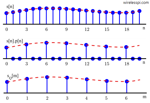
Downsampling is the process of reducing the sample rate by an integer factor. A signal $s[n]$ can be downsampled by a factor of $Q$ by retaining every $Q$th sample and discarding the remaining samples. The new slower sample rate is $1/Q$ of the original faster sample rate. The time and frequency domain visualizations of downsampling stages are now explained.

Time Domain View

---

• If the bandwidth of $s[n]$ is less than or equal to $1/Q$ of the original sample rate, a corresponding reduction in sample rate can be achieved by keeping the samples with indices $0$, $Q$, $2Q$, $\cdots $ and discarding $Q-1$ samples after each such retained sample.
• Such a process can be imagined as multiplying $s[n]$ with a sampling sequence $p[n]$ with period $Q$ and then throwing off the intermediate zero samples. In practice, such zero values are not computed through multiplication as they are immediately discarded.

A $3:1$ downsampling operation is graphically illustrated for time domain in Figure below.

Frequency Domain View

---

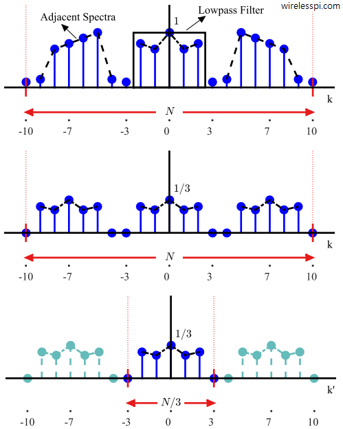
What happens in frequency domain is fairly interesting which can be explained with the help of $3:1$ downsampling operation graphically illustrated in Figure below.

• First, note that when we downsample a signal to a lower sample rate, there is a risk of going below the limit imposed by sampling theorem that can induce aliasing. Moreover, adjacent spectra might need to be cleaned up as well. For these reasons, we should apply a lowpass filter prior to downsampling which ensures that our signal contains no significant energy above the new lower sample rate.
• Next, in the discussion on convolution, we learned that multiplication in one domain is equivalent to convolution in the other domain. Here, multiplication in time between $s[n]$ and sampling sequence $p[n]$ with period $Q$ affects a convolution in frequency between $S[k]$ and $P[k]$ (there is an additional factor of $1/N$ for discrete signals, see some DFT properties). From the article on the DFT of a sampling sequence, the spectrum of $P[k]$ consists of $Q$ impulses at frequency bins $k=0$, and integer multiples of $k = \pm N/Q$. Furthermore, these spectral replicas are scaled down by a factor of $Q$. Finally, convolution of a signal with a unit impulse is the signal itself. Combining these facts, the result of this convolution is the emergence of $Q$ spectral copies of $S[k]$, one at frequency bin $k=0$ and others at $\pm N/Q$, all scaled down in spectral magnitude by $Q$.
• The final step is to reduce the bandwidth by a factor of $Q$, which in frequency domain is identical to throwing all the frequency bins except $N/Q$ samples around the bin $k=0$. The new spectral aliases appear around this range according to the new sample rate.

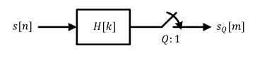
Block Diagram

---

A block diagram of filtering and downsampling is shown in Figure below. Here, $H[k]$ is the lowpass filter that limits the bandwidth of the initial signal $s[n]$ and cleans any neighboring spectra around it.

Effect on Peak Amplitude and Energy

---

A discussion about peak amplitude and energy as a result of downsampling operation is in order. We start with the Parseval relation that relates the signal energy in time domain to that in frequency domain.
\begin{equation}\label{eqCommSystemParsevalRelation}
E_s = \sum _{n=0} ^{N-1} |s[n]|^2 = \frac{1}{N} \sum _{n=0} ^{N-1} |S[k]|^2
\end{equation}

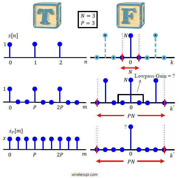
To make this discussion easier to follow, we refer to downsampling a rectangular signal of length $N$, which is also a complex sinusoid of frequency $0$. The DFT of such a signal is given by a unit impulse of height $N$ which was derived in DFT examples. The whole downsampling procedure for this signal is shown in Figure below, where the left and right columns are time and frequency domains, respectively.

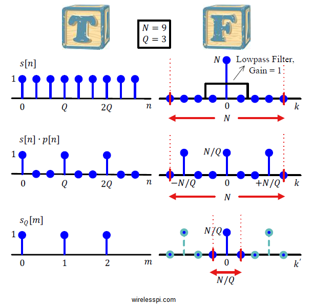
[Time] Notice from Figure above that the time domain amplitude of the samples of a downsampled signal remains unchanged.
\begin{equation}\label{eqIntroductionDownsamplingAmplitude}
\text{Amplitude}\left\{s_Q[m]\right\} = \text{Amplitude}\left\{s[n]\right\}
\end{equation}

However, the energy of the downsampled signal is lesser than the energy of the original signal due to discarding the intermediate samples. Assuming an amplitude of $A$, the energy in every $Q$ samples of $s[n]$ is $QA^2$. Since only $1$ out of every $Q$ samples remain in $s_Q[m]$, its energy in every $Q$ samples is $A^2$, a loss by a factor of $1/Q$. So
\begin{equation}\label{eqIntroductionDownsamplingEnergy}
E_{s_Q} = \frac{1}{Q}\cdot E_{s}
\end{equation}

Obviously, the relation is exact for this example, but approximate for realistic signals and gets more accurate with large number of samples.

[Frequency] To verify these results in frequency domain, consider from Parseval relation and top of above Figure that the energy in the actual signal is $(1/N)\cdot N^2 = N$. Also, recall from the DFT of the sampling sequence in DFT examples that its spectral impulses bear a reduction in value equal to $1/Q$. When a spectral shape is convolved with these impulses, the shape does get replicated at integer multiples of $k = N/Q$ but it bears a loss of spectral magnitude equal to $1/Q$ as well. The energy in this intermediate figure is $(1/N)\cdot Q (N/Q)^2$ $=$ $N/Q$, as in its time domain counterpart on the left. When we discard the neighboring spectra by reducing the sample rate, we essentially retain only $1/Q$ of the spectral energy. This is shown at the bottom of above Figure where owing to new signal length and DFT size $N/Q$ instead of $N$,
\begin{equation*}
E_{s_Q} = \frac{1}{N/Q}\cdot \frac{N^2}{Q^2} = \frac{N}{Q} = \frac{1}{Q} \cdot E_s
\end{equation*}

Upsampling

---

The procedure for upsampling a signal can be explained as a dual to downsampling.

Time Domain View

---

• Starting from a signal $s[n]$, the sample rate is increased by a factor of $P$ through inserting $P-1$ zero valued samples between the original input samples.
• In this new time axis, the original samples lie at indices $0$, $P$, $2P$, $\cdots$. These samples can be interpolated to obtain a smooth curve with increased sample rate.

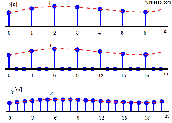
A $1:3$ upsampling operation is graphically illustrated for time domain in Figure below.

Frequency Domain View

---

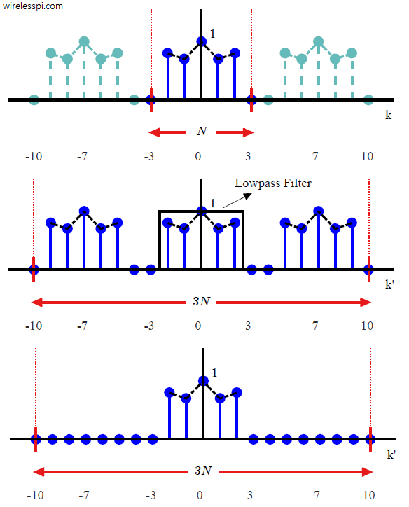
Let us turn our attention towards the frequency domain through a $1:3$ upsampling operation in Figure below.

• An increase in sample rate causes the primary zone to take in $P-1$ spectral copies at multiples of the original sample rate. Note the change in the dotted red lines since our primary zone is now changed.
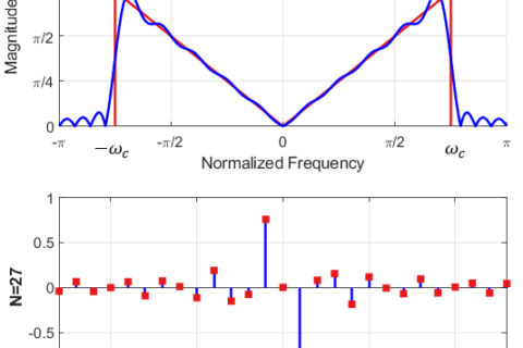
• A lowpass filter can now be employed to reject these $P-1$ spectral replicas leaving only the central spectrum. This filtering has the effect of interpolating between the samples in time domain (since we are convolving with a sinc function in time domain).

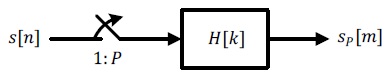
Block Diagram

---

A block diagram of upsampling and filtering is shown in Figure below. Here, $H[k]$ is the lowpass filter that rejects the neighboring spectra around the central spectrum.

Effect on Peak Amplitude and Energy

---

As with downsampling, a discussion about peak amplitude and energy as a result of upsampling operation is in order. Again, we refer to upsampling a rectangular signal of length $N$, which is also a complex sinusoid of frequency $0$ with height $N$. The whole upsampling procedure for this signal is shown in Figure below, where the left and right columns are time and frequency domains, respectively.

[Time] Notice from above Figure that the energy to raise the intermediate samples from dead has to come from somewhere. Effectively, this comes from the original non-zero samples whose energy gets spread out to all $P$ samples. As a result, the time domain amplitude of the samples of an upsampled signal gets reduced to $x$, which is unknown at this stage.

Next, the energies in both the original and zero-inserted signal are the same, $E_s=N$. To relate it to the energy of the upsampled signal, note that
\begin{equation*}
E_{s_P} = \underbrace{x^2 + x^2 + \cdots x^2}_{\text{PN terms}} = PN \cdot x^2
\end{equation*}
If we want to have the same energy as before,
\begin{align*}
E_{s_P} &= E_s \quad \Rightarrow \quad PN x^2 = N \\
x &= \frac{1}{\sqrt{P}} \quad \text{for equal energies $E_s$ and $E_{s_P}$}
\end{align*}

[Frequency] Now recall Parseval relation and consider from the top of above Figure in frequency domain that the energy in the actual signal is $(1/N)\cdot N^2 = N$. When the sample rate is increased, the signal length and DFT size increases from $N$ to $PN$ and the energy in the intermediate figure is again $1/(PN)\cdot P \cdot N^2$ $=$ $N$, as is in its time domain counterpart on the left. Finally, we try three possible gains for the lowpass filter: $1$, $\sqrt{P}$ and $P$. Then, the energy in the lowpass filtered spectrum at the bottom of above Figure is
\begin{align}
E_{s_P} = \frac{1}{PN}\cdot N^2 = \frac{N}{P} &= \frac{1}{P} \cdot E_s \quad \text{for a filter gain = $1$} \nonumber \\
E_{s_P} = \frac{1}{PN}\cdot (\sqrt{P} N)^2 = N &= E_s \quad \text{for a filter gain = $\sqrt{P}$} \nonumber \\
E_{s_P} = \frac{1}{PN}\cdot (PN)^2 = PN &= P \cdot E_s \quad \text{for a filter gain = $P$} \label{eqIntroductionUpsamplingEnergy}
\end{align}

In the above derivations, we used the fact that the definition of energy in frequency domain has a factor of horizontal span in the denominator. This horizontal span is $PN$ instead of $N$ for upsampled signal. Also, the relations are approximate for realistic signals and get more accurate with increasing number of samples.

The final task is to find $x$ in time domain of the upsampled signal which can be found by noting that

• Energy in upsampled time domain signal is $PNx^2$.
• Energies in time and frequency domains for their respective filter gains at the bottom of above Figure should be equal.

Accordingly, for gain equal to $1$,
\begin{align*}
PNx^2 &= \frac{N}{P} \\
x &= \frac{1}{P} \quad \text{for a filter gain = $1$}
\end{align*}
for gain equal to $\sqrt{P}$,
\begin{align*}
PNx^2 &= N \\
x &= \frac{1}{\sqrt{P}} \quad \text{for a filter gain = $\sqrt{P}$}
\end{align*}
and for gain equal to $P$,
\begin{align}
PNx^2 &= PN \nonumber \\
x &= 1 \quad \text{for a filter gain = $P$} \label{eqIntroductionUpsamplingAmplitude}
\end{align}

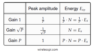
The question is: which filter gain is the best choice? There is no definite answer as this choice depends on the application. To maintain the same energy, the gain should be $\sqrt{P}$. However, to maintain the same peak time domain amplitude in the upsampled signal as before, the filter should be designed with gain $P$. In most applications, maintaining the same peak amplitude after increasing the sample rate is the target.

These results are summarized in Table below.