For understanding what follows, we need to refer to the Discrete Fourier Transform (DFT) and the effect of time shift in frequency domain first. Here, we discuss a few examples of DFTs of some basic signals that will help not only understand the Fourier transform but will also be useful in comprehending concepts discussed further.
A Rectangular Signal
A rectangular sequence, both in time and frequency domains, is by far the most important signal encountered in digital signal processing. One of the reasons is that any signal with a finite duration, say $T$ seconds, in time domain (that all practical signals have) can be considered as a product between a possibly infinite signal and a rectangular sequence with duration $T$ seconds. This is called windowing and a rectangular sequence is the simplest form of a window. Windowing is a key concept in implementation of many DSP applications.
Let us compute the $N$-point DFT of a length-$L$ rectangular sequence
\begin{equation}\label{eqIntroductionRectangular}
s_I[n] = \left\{ \begin{array}{l}
1, \quad n_s \le n \le n_s+L-1 \\
0, \quad \text{otherwise} \\
\end{array} \right.
\end{equation}
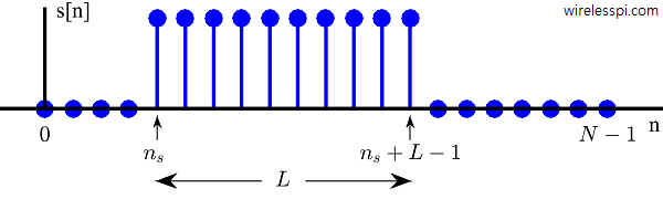
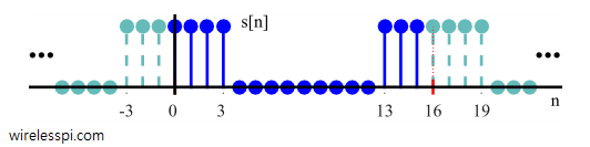
shown in Figure below, where $N \ge L$.
Since this sequence is real with no $Q$ component in time domain, the $I$ component in frequency domain from DFT definition can be expressed as
\begin{align}
S_I[k] &= \sum \limits _{n=n_s} ^{n_s+L-1} s_I[n] \cos 2\pi\frac{k}{N}n \nonumber \\
&= \sum \limits _{n=n_s} ^{n_s+L-1} \cos 2\pi\frac{k}{N}n \label{eqIntroductionDerivation1} \\
&= \sum \limits _{n=n_s} ^{n_s+L-1} \cos 2\pi\frac{k}{N}n~ \frac{\sin \pi\frac{k}{N}}{\sin \pi\frac{k}{N}} \nonumber
\end{align}
Let $\theta = 2\pi k/N$ and using the identity $\cos(A)\sin(B) = 0.5 \{ \sin(A+B) – \sin(A-B) \}$, we get
\begin{align*}
S_I[k] &= \sum \limits _{n=n_s} ^{n_s+L-1} \cos n\theta~ \frac{\sin \theta/2}{\sin \theta/2} \\
&= \frac{1}{2\sin \theta/2} \sum \limits _{n=n_s} ^{n_s+L-1} \left[ \sin \left( n+\frac{1}{2}\right)\theta – \sin \left( n-\frac{1}{2}\right)\theta \right] \\
&= \frac{1}{2\sin \theta/2} \left[ \sin \left( n_s+L-\frac{1}{2}\right)\theta – \sin \left( n_s-\frac{1}{2}\right)\theta \right] \\
\end{align*}
where all the other terms in the summation cancel out. Using the same identity as above
\begin{align*}
S_I[k] &= \frac{1}{\sin \theta/2} \cos \left(n_s + \frac{L-1}{2}\right)\theta \cdot \sin\left(\frac{L}{2} \right)\theta \\
&= \frac{\sin L \theta/2}{\sin \theta/2} \cos \left(n_s + \frac{L-1}{2}\right)\theta \nonumber
\end{align*}
Plugging in the expression back for $\theta$,
\begin{align}
S_I[k] &= \frac{\sin \pi L k/N}{\sin \pi k/N} \cos \left[ 2\pi \frac{ k}{N}\left(n_s + \frac{L-1}{2}\right) \right]\label{eqIntroductionDFTrectangleI}
\end{align}
Similarly, $Q$ component can be found from DFT definition,
\begin{align*}
S_Q[k] &= \sum \limits _{n=n_s} ^{n_s+L-1} -s_I[n] \sin 2\pi\frac{k}{N}n \\
&= \sum \limits _{n=n_s} ^{n_s+L-1} -\sin 2\pi\frac{k}{N}n
\end{align*}
Following the same procedure as $I$ component, and using the identity $\sin(A)\sin(B) = \frac{1}{2}$ $\left\{ \cos(A-B) -\right.$ $\left. \cos(A+B) \right\}$, the $Q$ component of its DFT is given by
\begin{align}
S_Q[k] &= -\frac{\sin \pi L k/N}{\sin \pi k/N} \sin\left[ 2\pi\frac{k}{N} \left(n_s + \frac{L-1}{2}\right) \right]\label{eqIntroductionDFTrectangleQ}
\end{align}
Despite its simplicity, there is a lot of information hidden and several interesting conclusions to be drawn here for which we continue further discussion below.
Magnitude and Phase
Applying the definitions of magnitude and phase to Eq \eqref{eqIntroductionDFTrectangleI} and Eq \eqref{eqIntroductionDFTrectangleQ} and using $\cos^2 A + \sin^2 A = 1$, we get the magnitude and phase of the DFT of a rectangular signal.
\begin{equation}
|S[k]| = \frac{\sin \pi L k/N}{\sin \pi k/N} \label{eqIntroductionDFTrectangleM}
\end{equation}
\begin{equation}
\measuredangle S[k] = -2\pi\frac{k}{N} \left(n_s + \frac{L-1}{2}\right) \label{eqIntroductionDFTrectangleP}
\end{equation}
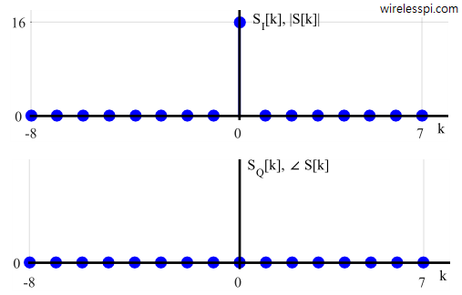
The above Figure displays the magnitude and phase plots for the DFT of a rectangular signal with $L=N=16$ which in this case are similar to the $I$ and $Q$ plots, respectively. In general, magnitude-phase and $IQ$ plots convey different information, many examples of which we will encounter throughout this text. In most situations, magnitude-phase plot delivers a great deal of information while in some others, $IQ$ plot is more relevant.
DFT, Frequency Domain Sampling and Leakage
For DFT of a rectangular signal, the $IQ$ equations are given in Eq \eqref{eqIntroductionDFTrectangleI} and Eq \eqref{eqIntroductionDFTrectangleQ}, and the magnitude-phase equations in Eq \eqref{eqIntroductionDFTrectangleM} and Eq \eqref{eqIntroductionDFTrectangleP}. The corresponding figures are drawn in the Figure above with single impulses at bin 0.
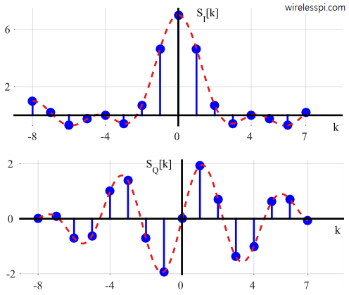
The question is: How can such complex equations generate such simple figures? The answer is that it was a special case due to the whole sequence being equal to one. For an $L$ < $N$ and using Eq \eqref{eqIntroductionDFTrectangleP}, the rectangular signal can be made symmetric around zero position, as shown in Figure below for $L = 7$, $N = 16$ and $n_s = -(L-1)/2$ (which is the same as $n_s = N -(L-1)/2$ due to DFT input periodicity.
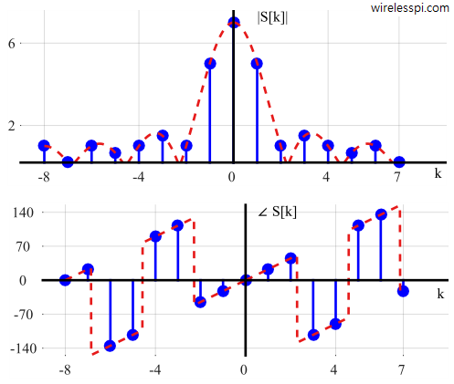
Now consider the case of $L = 7$, $N = 16$ and $n_s = -(L-1)/2-1 = -4$. The sequence can be imagined as shifted to the left by $1$ from its symmetric position around zero. $I$ and $Q$ plots from Eq \eqref{eqIntroductionDFTrectangleI} and Eq \eqref{eqIntroductionDFTrectangleQ} are shown in Figure below.
Similarly, the magnitude and phase plots from Eq \eqref{eqIntroductionDFTrectangleM} and Eq \eqref{eqIntroductionDFTrectangleP} are plotted in Figure below.

A clear shape of sinc function in terms of $\sin (\pi L k/N)$ $/$ $\sin (\pi k/N)$ is visible in magnitude plot which is sampled at discrete frequencies $k/N$. Now we can recognize that the plots in the earlier figure were also sinc functions but sampled at the peak value at bin $0$ and at zero crossings for all other bins.
To comprehend the reason why energy appeared in other frequency bins as well, consider that as explained in the article about complex numbers, a complex sinusoid is composed of $\cos(\cdot)$ and $\sin(\cdot)$ as $I$ and $Q$ components, respectively. These $\cos(\cdot)$ and $\sin(\cdot)$ are orthogonal to each other over a complete period, and $\cos(\cdot)$ ($\sin(\cdot)$) of one frequency $k/N$ is also orthogonal to $\cos(\cdot)$ ($\sin(\cdot)$) of other frequencies $k’/N$, provided that $k’$ are also integers, i.e.,
\begin{equation}
\begin{aligned}
\sum \limits _{n=0} ^{N-1} \cos 2\pi \frac{k}{N}n \cdot \sin 2\pi \frac{k}{N}n = 0 \nonumber\\
\sum \limits _{n=0} ^{N-1} \cos 2\pi \frac{k}{N}n \cdot \cos 2\pi \frac{k’}{N}n = 0 \label{eqIntroductionOrthogonality}\\
\sum \limits _{n=0} ^{N-1} \sin 2\pi \frac{k}{N}n \cdot \sin 2\pi \frac{k’}{N}n = 0 \nonumber
\end{aligned}
\end{equation}
The DFT finds the contributions of analysis frequencies $F = F_S \cdot k/N$ for for $k = -N/2$, $\cdots,-1,0,1,$ $\cdots,N/2-1$ in an input signal, which are all integer multiples of a fundamental frequency $F_S/N$. It is due to this integer multiplicity that DFT is able to find each $k-th$ contribution independently of all others. And if the input signal contains contributions from only these frequencies, the DFT output is proportional to the magnitude at the contributing frequency bins and zero at the remaining bins.
In a real scenario, the input data sequence is not bound to contain energy precisely at a set of given analysis frequency bins. If the input has a signal component at some intermediate frequency between these integer multiples of $F_S/N$, say $1.3 F_S /N$, the orthogonality does not hold and this input signal shows up to some degree in all $N$ output bins of our DFT due to unaligned sampling instants in frequency domain. This is known as DFT leakage.
When we perform the DFT on real-world finite-length time sequences, DFT leakage is an unavoidable phenomenon. Let us construct an example to observe this in detail.
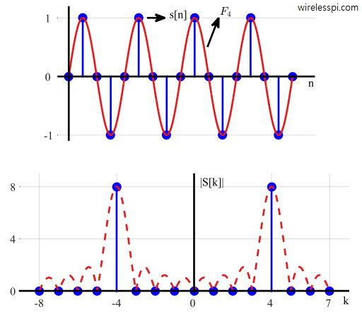
Assume a signal with frequency $4$ kHz at a sample rate of $F_S = 16$ kHz.
\begin{align*}
s[n] = \sin 2\pi \frac{4}{16} n
\end{align*}
The solid blue curve is shown in Figure above in time domain along with one analysis frequency $F_4 = F_S \cdot k/N = 16000 \cdot 4/16 = 4$ kHz. Note that both the input frequency and the analysis frequency $F_4$ complete four full cycles during the sampling interval and hence its DFT, plotted in Figure above, has two impulses at bins $4$ and $-4$ with zero input from all the other bins. The shape of the actual curve is the same sinc function but it is sampled in frequency domain at just the right points — integer frequency bins due to integer number of cycles of the input in time domain.
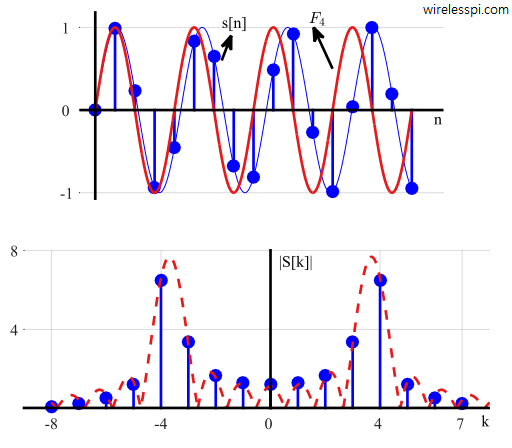
Now let us change the input signal slightly by making the input frequency equal to $3.7$ kHz as shown in Figure below.
\begin{align*}
s[n] = \sin 2\pi \frac{3.7}{16} n
\end{align*}
Observe in this Figure below that the analysis frequency $F_4$ completes four full cycles during that interval, while the frequency $3.7$ kHz in the original signal $s[n]$ does not have integer number of cycles over $16$-sample interval, causing the input energy to leak into all the other DFT output bins. The $k = 3$ bin is not zero because the sum of the products of the input sequence and the $k = 3$ analysis frequency is no longer zero (same is also true for, say, $k=4$). This leakage causes any input signal whose frequency is not exactly at a DFT bin center to leak into all of the other DFT output bins. The shape of the sinc function did not change as compared to a $4$ kHz input but it is sampled in frequency domain at non-ideal points — fractional frequency bins due to non-integer number of cycles of the input in time domain.
One final question: an input sinusoid at $3.7$ kHz sampling the sinc function at unaligned points in frequency domain makes sense, but why the graph in the earlier figure exhibits a similar kind of leakage? The reason is that an all-ones rectangular sequence with $L=N=16$ can be considered a single complex sinusoid at frequency $0$ but its truncated version with $L = 7$, $N=16$ is not. It is actually made up of all $N$ sinusoids just like a periodic square wave.
Mainlobe Peak
The DFT of a rectangular signal has a mainlobe centered about the $k = 0$ point. Its amplitude cannot be found by plugging in $k=0$ in Eq \eqref{eqIntroductionDFTrectangleM} because both the numerator and denominator become zero resulting in undefined $0/0$ expression. Although a mathematical trick (known as L’Hôpital’s rule) can be applied to compute it mathematically, we take an easier course. The peak amplitude of the mainlobe is $L$ because at $k = 0$, DFT definition dictates that the DFT $S[0]$ is the sum of all original samples due to $\cos 2\pi (k/N) n = 1$ and $\sin 2\pi (k/N) n = 0$. Then, the sum of $L$ unity-valued samples is $L$. Consequently, the peak value is seen to be $L = 16$ and $L = 7$ in their respective figures.
Mainlobe Width and Zero Crossings
The width of the mainlobe is defined by zero crossings of the curve. Since $\sin \pm \pi = 0$, the first zero crossing occurs when the numerator argument in Eq \eqref{eqIntroductionDFTrectangleM}, $\sin \pi L k/N$, is equal to $\pi$. All other zero crossings are integer multiples of the first. So the mainlobe width is given by the value of the first zero crossing $k_{zc}$ as
\begin{align*}
\pi L \frac{k_{zc}}{N} &= \pi \\
k_{zc} &= \frac{N}{L}
\end{align*}
This value is confirmed from $N/L = 1$ and $N/L = 16/7 = 2.29$ in their respective figures. A zero crossing right at sample $1$ illustrates that it was sampled at peak value for bin $0$ and at zero for all other bins.
DFT Phase
Most of the discussion until now was around the magnitude plots. Let us understand the concept of phase again through the DFT of a rectangular signal. Now the phase plot for $L=7$, $N=16$ and $n_s=-(L-1)/2-1$ has been drawn in Figure below after unwrapping $180^\circ$ phase jumps which arose due to changing $I$ and $Q$ signs. The resulting phase is a straight line with a positive slope equal to $22.5^\circ$. Where did this number come from?
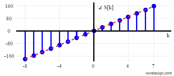
We learned before that a time shift of $n_0$ samples results in phase rotation of $\Delta \theta (k) = 2\pi (k/N) n_0$, the direction of which depends on the direction of time shift. For time traveling in the past (i.e., a signal delay), the phase rotation is also negative while for time traveling in the future (i.e., a signal advance), the phase rotation is also positive.
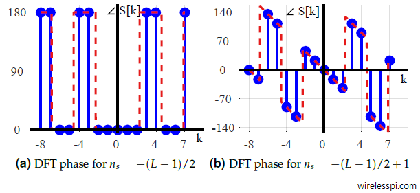
To complete the picture, we need one extra piece of information that we prove later: the DFT of a real and even symmetric signal is purely real with $0$ $Q$ part. Consequently, its phase is equal to $0$ or $\pi$ (depending on the sign of $I$ part). In our example, an even symmetric signal would have been obtained for $n_s=-(L-1)/2$. Then, the phase plot would be $0$ or $\pi$ as shown in Figure (part a) below.
However, for $n_s = -(L-1)/2-1$, it is a left shift of that even symmetric signal by $1$ sample. Thus, plugging $n_0=+1$ in the expression $2\pi (k/N) n_0$ gives the phase rotation $\theta (k)$ for each frequency bin as
\begin{align*}
\Delta \theta(k) &= 2\pi \frac{k}{N} n_0 \\
&= 2\pi \frac{k}{N}, \quad k = -N/2,\cdots,-1,0,1,\cdots,N/2-1
\end{align*}
In this case, $N$ was equal to $16$. Starting from $k = 0$, the phase shift can be seen to be $0$. For all $k$,
\begin{align*}
\Delta \theta(0) &= 2\pi \frac{0}{N} \times \frac{180^\circ}{\pi} = 0 \\
\Delta \theta(\pm1) &= 2\pi \frac{\pm1}{N} \times \frac{180^\circ}{\pi} = \pm 22.5^\circ \\
\Delta \theta(\pm2) &= 2\pi \frac{\pm2}{N} \times \frac{180^\circ}{\pi} = \pm 45 ^\circ \\
\Delta \theta(\pm3) &= 2\pi \frac{\pm3}{N} \times \frac{180^\circ}{\pi} = \pm 67.5^\circ \\
&\cdots \\
&\cdots
\end{align*}
A linear slope of $22.5^\circ$ is thus verified. Part (b) of above Figure shows the phase plot for a right shift of $1$, i.e., $n_s = -(L-1)/2+1$. Observe a negative slope of $-22.5^\circ$ when adjusted for $180^\circ$ phase jumps.
A General Sinusoid
The DFT of a general sinusoid can be derived similarly by plugging the expression of a complex sinusoid in DFT definition and following the same procedure as in the rectangular sequence example, as done here.
Nevertheless, having understood the above concepts, we can see how the magnitude and phase plots of the DFT of a general sinusoid look like by an easier method. As an all-ones rectangular sequence is nothing but a complex sinusoid with frequency $0$ with length $L=N$, the DFT magnitude of a general complex sinusoid with frequency $k’$ (which can be a non-integer) can be found by putting $L=N$ (as it spans the whole length), $n_s=0$ (as it starts at $0$) and $k-k’$ instead of $k$ in Eq \eqref{eqIntroductionDFTrectangleM} and Eq \eqref{eqIntroductionDFTrectangleP} as
$$\begin{equation}
\begin{aligned}
|S[k]| &= \frac{\sin \pi (k-k’)}{\sin \pi (k-k’)/N} \\
\measuredangle S[k] &= -2\pi\frac{k-k’}{N} \left(\frac{N-1}{2}\right)
\end{aligned}
\end{equation}\label{eqIntroductionDFTgeneralSinusoid}$$
Similarly, the DFT of a real sinusoid $\cos[2\pi (k’/N)n]$ can be seen as the sum of the above expression with a similar expression replacing $k-k’$ with $k+k’$ because each real sinusoid consists of two complex sinusoids scaled by half.
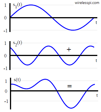
For example, consider a signal shown in Figure below and consisting of two sinusoids at $1$ kHz and $2$ kHz as
\begin{align*}
s(t) &= s_1(t) + s_2(t) \\
&= \sin(2\pi 1000 t) + 0.75\sin(2\pi 2000 t + 120 ^\circ)
\end{align*}
It can be seen that $s[n]$ has only an $I$ component with zero $Q$ component. Sampling the above signal at a rate of $1/T_S = F_S = 8$ kHz produces
$$\begin{equation}
\begin{aligned}
s[n] &= \sin(2\pi 1000 nT_S) + 0.75\sin(2\pi 2000 nT_S + 120^\circ) \nonumber \\
&= \sin\left(2\pi \frac{1}{8}n\right) + 0.75\sin\left(2\pi \frac{2}{8}n + 120^\circ \right)
\end{aligned}
\end{equation}\label{eqIntroductionDFTPhaseExample}$$
Our DFT analysis frequencies for an $8$ point DFT are
\begin{align*}
F &= F_S \cdot \frac{k}{N} \\
k = 0 &\Rightarrow 8000 \cdot\frac{0}{8} = 0~ \text{kHz} \\
k = \pm1 &\Rightarrow 8000 \cdot\frac{\pm1}{8} = \pm1~ \text{kHz} \\
k = \pm2 &\Rightarrow 8000 \cdot\frac{\pm2}{8} = \pm2~ \text{kHz} \\
k = \pm3 &\Rightarrow 8000 \cdot\frac{\pm3}{8} = \pm3~ \text{kHz} \\
\end{align*}
So in this case, bin $1$ corresponds to an actual frequency of $1$ kHz, bin $2$ to $2$ kHz, and so on. The DFT $S[k]$ can be found by applying the DFT definition and is plotted in Figure below.
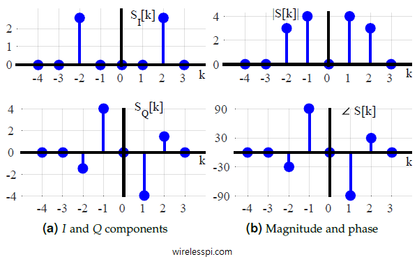
From magnitude plot of this figure, observe that the DFT has detected two real sinusoids in this signal because the impulses at bins $1$ and $-1$ indicate the presence of two complex sinusoids that combine to form one real sinusoid at a frequency $8000\cdot1/8 = 1$ kHz. A similar argument holds for the other frequency of $2$ kHz.
DC or Average Value
The DC, or average, value of this signal $\frac{1}{N}\sum s[n] $ is $0$ which is evident from Eq \eqref{eqIntroductionDFTPhaseExample} as the average value of a sinusoid over an integral number of cycles is $0$.
Magnitude
When an input signal contains a complex sinusoid of peak amplitude $A$ with an integral number of cycles over $N$ input samples, the output magnitude of the DFT for that particular sinusoid is $AN$. This can be checked by plugging in the expression for a complex sinusoid into DFT definition. Using orthogonality, the DFT output for a complex sinusoid is given as
\begin{align*}
\sum \limits _{n=0} ^{N-1} \cos 2\pi \frac{k}{N}n \cdot \cos 2\pi \frac{k}{N}n + \sin 2\pi \frac{k}{N}n \cdot \sin 2\pi \frac{k}{N}n \\
\sum \limits _{n=0} ^{N-1} \sin 2\pi \frac{k}{N}n \cdot \cos 2\pi \frac{k}{N}n – \cos 2\pi \frac{k}{N}n \cdot \sin 2\pi \frac{k}{N}n
\end{align*}
Using the identities $\cos A \cos B$ $+$ $\sin A \sin B$ $=$ $\cos (A-B)$ and $\sin A$ $\cos B$ $-$ $\cos A \sin B$ $=$ $\sin (A-B)$,
\begin{align*}
\sum \limits _{n=0} ^{N-1} \cos 0 &= N \\
\sum \limits _{n=0} ^{N-1} \sin 0 &= 0
\end{align*}
Thus, the output magnitude of the DFT is proved as $AN$.
For a real sinusoid, $s_Q[n]$ is $0$ and only the first term in $I$ part of the above equation survives. Since $\cos^2 A = 1/2(1+\cos 2A)$, the output magnitude of the DFT for a real sinusoid is $AN/2$.
Considering the fact that $s[n]$ is composed of two real sine waves with amplitudes $1$ and $0.75$, we can see that $1$ kHz sine wave has a magnitude $1\times N/2 = 4$ and $2$ kHz sine wave has a magnitude $0.75 \times N/2 = 3$.
But if the sinusoid in a rectangular signal is real with frequency $0$, why is the peak value in the magnitude plot equal to $N = 15$ rather than $N/2 = 7.5$? This is because the DFT of a regular real sinusoid is two impulses with amplitude $N/2$, one at that frequency and the other at its negative counterpart, but at frequency $0$, both of these impulses merge together to give a magnitude of $N$. Another way to understand it is that an all-ones sequence is actually a complex sinusoid at frequency $0$ because it has an all-ones sequence in $I$ part and all-zeros sequence in $Q$ part.
\begin{align*}
\cos 2\pi \frac{k}{N}n &= \cos 2\pi \frac{0}{N}n = 1, \quad\quad n = 0,\cdots,N-1\\
\sin 2\pi \frac{k}{N}n &= \sin 2\pi \frac{0}{N}n = 0, \quad\quad n = 0,\cdots,N-1
\end{align*}
Phase
Referring to the phase plot and going back to the DFT definition, assume that the input is $\cos 2\pi (k/N) n$. The DFT output is given as
\begin{align*}
\sum \limits _{n=0} ^{N-1} \cos 2\pi \frac{k}{N}n \cdot \cos 2\pi \frac{k}{N}n + 0 \cdot \sin 2\pi \frac{k}{N}n &= a\\
\sum \limits _{n=0} ^{N-1} 0 \cdot \cos 2\pi \frac{k}{N}n – \cos 2\pi \frac{k}{N}n \cdot \sin 2\pi \frac{k}{N}n &= 0
\end{align*}
for an arbitrary number $a$ and orthogonality of $\cos(\cdot)$ and $\sin(\cdot)$ over a complete period. The phase is $\tan^{-1} (0/a) = 0$ for positive $a$ and $\tan^{-1} 0/-a + \pi = \pi$ for negative $a$. Therefore, a $0$ phase at a particular frequency $F = F_S \cdot k/N$ is with respect to a cosine wave at that same frequency.
The bin $1$ frequency at $8000 \cdot 1/8 = 1$ kHz has a phase of $-90 ^\circ$. Is it a cosine with a phase of $-90^\circ$? From the identity $\cos (A-90^\circ) = \sin (A)$, it is indeed a sine waveform with an initial phase of $0$ which can be confirmed from the first term $\sin 2\pi (1/8)n$ of $s[n]$ in Eq \eqref{eqIntroductionDFTPhaseExample}. The corresponding phase at bin $-1$ is obviously $-(-90^\circ)=+90 ^\circ$.
As for the second term $0.75 \sin\left\{ 2\pi (2/8)n + 120^\circ\right\}$, it is a sine at $2$ kHz with a phase shift of $120 ^\circ$, or a cosine with a phase of $120^\circ-90^\circ = 30 ^\circ$.
Notice in the DFT how the signal is composed of two sinusoids at $1$ and $2$ kHz, respectively, where former is a cosine with a phase of $-90^\circ$ (or a sine with $0^\circ$) and the latter is a cosine with a phase of $30^\circ$ (or a sine with $120^\circ$). Now referring to its time domain plot, the first sinusoid $s_1(t)$ is positioned around the origin according to its $-90^\circ$ cosine (or $0^\circ$ sine) phase, while the second sinusoid $s_2(t)$ is positioned around the origin according to its $30^\circ$ cosine (or $120^\circ$ sine) phase. Through the phase plot, the DFT in fact finds the time alignments of all the sinusoids at bin frequencies $F_S \cdot k/N$.
Sometimes it is easy to get confused from the fact that $Q$ component of $s[n]$ is $0$ in the above example, leading to an incorrect phase result of $0$ or $\pi$. However, we have to differentiate $IQ$-plane of time domain from $IQ$-plane of frequency domain. The $Q$ component here is $0$ in time domain only but the phase plot is determined by $IQ$ components in frequency domain. There, a real sinusoid is a sum of two complex sinusoids and the phase of those two complex sinusoids in frequency $IQ$-plane determines the starting sample of the real sinusoid in time domain.
Do remember that the plots are — once again — sinc functions overlapping each other. However, since the signal consists of two exact analysis frequencies, the frequency domain is sampled at the precise locations of zero crossings. That being the case, the sinc function becomes invisible and looks like two sets of impulses only.
The Unit Impulse
Having known the DFT of a rectangular signal, we have two ways to find the Fourier transform of a unit impulse.
[Time-Frequency Duality] A closer look at DFT and iDFT equations reveal that the forward and inverse transform are almost identical, except the scaling factor $1/N$ and direction of rotations of analysis sinusoids. Therefore, time and frequency domains are dual and DFT of a signal in time domain can be derived by the iDFT of a signal in frequency domain. For example, a single impulse at frequency bin $0$ is an all-ones rectangular sequence in time domain. By duality, the inverse is also true: a single impulse in time domain corresponds to an all-ones rectangular sequence in frequency domain.
[Rectangular signal] From a general rectangular sequence, it is evident that a unit impulse is also a rectangular sequence with length $L = 1$. Therefore,
\begin{align}
|S[k]| &= \frac{\sin \pi k/N}{\sin \pi k/N} = 1 \label{eqIntroductionDFTunitImpulseM}
\end{align}
Since the starting sample $n_s = 0$, the angle is equal to $0$.
The Sampling Sequence
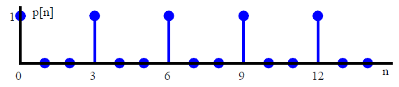
The sampling sequence is a sequence of unit impulses repeating with a period $M$ within our observation window (and owing to DFT input periodicity, outside the observation window as well). Figure below illustrates the sampling sequence in time domain for $M=3$ and $N=15$.
To compute its DFT, consider that $p_I[n] = p[n]$ and $p_Q[n]=0$. Then,
\begin{align*}
P_I[k] &= \sum \limits _{n=0} ^{N-1} p[n] \cos 2\pi\frac{k}{N}n
\end{align*}
Since $p[n]=0$ except when $n=M$, we can write $p[Mm] = 1$ where $m=0,1,\cdots,N/M-1$. We are assuming $N/M$ as an integer here because otherwise $p[n]$ will not be periodic. So in the above example, $m = 0,1,2,3,4$ for non-zero values of $n$ at $0, 3, 6, 9$ and $12$.
\begin{align*}
P_I[k] &= \sum \limits _{m=0} ^{N/M-1} \cos 2\pi\frac{k}{N} M m = \sum \limits _{m=0} ^{N/M-1} \cos 2\pi\frac{k}{N/M} m
\end{align*}
Note that the above equation is very similar to Eq \eqref{eqIntroductionDerivation1} encountered while computing the DFT of a rectangular sequence. Therefore, substituting both the length of the sequence $L$ and observation window $N$ equal to $N/M$ in Eq \eqref{eqIntroductionDFTrectangleM} and doing the same for $Q$ part, we get
\begin{align}
|P[k]| &= \frac{\sin \pi k}{\sin \pi k M/N} \label{eqIntroductionDFTSamplingSeqM}
\end{align}
Magnitude and Phase
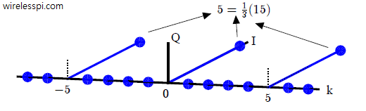
The sequence is plotted in frequency domain in Figure below, where both $I$ and $Q$ components are shown for $M = 3$ and $N=15$. Since the sequence is aligned in time such that it is symmetric with respect to zero, the phase is zero in frequency domain. So the magnitude plot is the same as the $I$ part.
Mainlobe Peak
In the DFT of a rectangular signal, we saw that both the numerator and denominator become equal to zero for $k=0$. In that case, the peak of the mainlobe was equal to $L$, the length of the sequence. We found this value by plugging $k=0$ in the DFT definition and deduced that the result is just a sum of all time domain samples because $\cos 2\pi k/N = 1$ and $\sin 2\pi k/N = 0$. Here in this case, the peak value can easily be seen as the sum of $N/M$ unit impulses and hence equal to $N/M = 5$.
Remember from DFT of a general sinusoid derived above that the DFT of a complex sinusoid with amplitude $A$ in time has a magnitude $AN$ in frequency domain. Here, the spectral replicas have a peak magnitude of $5$ instead of $15$ which suggests that the actual spectrum has been scaled down by a factor of $1/M=1/3$. This is shown in Figure above.
Mainlobe Positions
There are multiple impulses in frequency domain here: more than one as in DFT of an all-ones rectangular sequence but less than $N$ as in the DFT of a unit impulse. Observe from Eq \eqref{eqIntroductionDFTSamplingSeqM} that when the denominator is non-zero, the spectrum is clearly zero. When both the numerator and denominator are zero, the peak values are $N/M$ as above. To find these locations, check where the denominator is an integer multiple of $\pi$ as well.
\begin{align*}
\pi k_{\text{peak}} \frac{M}{N} &= \text{integer} \cdot \pi \\
k_{\text{peak}} &= \text{integer} \cdot \frac{N}{M}
\end{align*}
In our example, these peaks turn out to be $0$ and $\pm 5$ as shown in Figure above. If you guessed that these impulses in frequency domain are actually sinc functions sampled at just the peak and zero values, you are right (compute a length-$32$ DFT of this sequence instead of length-$15$, for example).
A Shifted Sampling Sequence
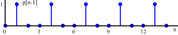
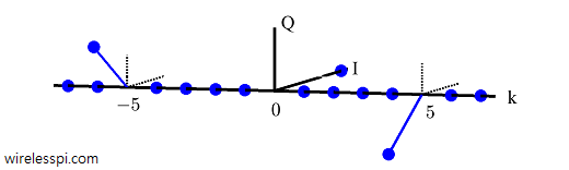
What happens when the sampling sequence studied above is shifted by one or more samples. From the effect of time shift in frequency domain, we know that a shifting a signal in time domain produces a multiplication of its spectrum with a complex sinusoid with inverse period equal to that shift. Subsequently, we can see the DFT of a right shifted by $1$ sampling sequence in the Figure below where the phase shift can be recognized as
\begin{equation*}
\pm 2\pi \frac{k}{N}n_0 = \pm 2\pi \frac{5}{15}(-1) = \mp 120 ^{\circ}
\end{equation*}
Concluding Remarks
To test some of your own signals and see the corresponding spectra, you can see the code here.
Finally, instead of finding the spectrum that consists of all the frequencies in DFT, we are sometimes interested in the magnitude of one particular frequency in the signal. Computing a DFT becomes inefficient in that case. See the Goertzel algorithm as a great example of how to solve this problem.