Convolution

Understanding convolution is the biggest test DSP learners face. After knowing about what a system is, its types and its impulse response, one wonders if there is any method through which an output signal of a system can be determined for a given input signal. Convolution is the answer to that question, provided that the system is linear and time-invariant (LTI).

We start with real signals and LTI systems with real impulse responses. The case of complex signals and systems will be discussed later.

Convolution of Real Signals

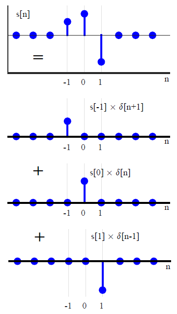
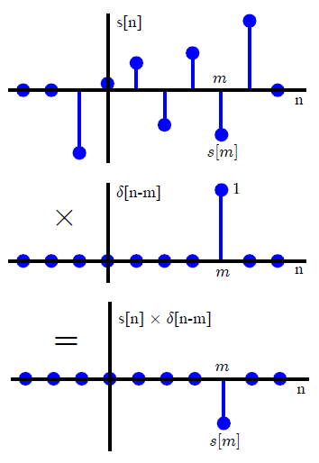
Assume that we have an arbitrary signal $s[n]$. Then, $s[n]$ can be decomposed into a scaled sum of shifted unit impulses through the following reasoning. Multiply $s[n]$ with a unit impulse shifted by $m$ samples as $\delta[n-m]$. Since $\delta[n-m]$ is equal to 0 everywhere except at $n=m$, this would multiply all values of $s[n]$ by 0 when $n$ is not equal to $m$ and by 1 when $n$ is equal to $m$. So the resulting sequence will have an impulse at $n=m$ with its value equal to $s[m]$. This process is clearly illustrated in Figure below.

This can be mathematically written as
\begin{equation*}
s[n] \delta [n-m] = s[m] \delta [n-m]
\end{equation*}
Repeating the same procedure with a different delay $m’$ gives
\begin{equation*}
s[n] \delta [n-m’] = s[m’] \delta [n-m’]
\end{equation*}

The value $s[m’]$ is extracted at this instant. Therefore, if this multiplication is repeated over all possible delays $-\infty < m < \infty$, and all produced signals are summed together, the result will be the sequence $s[n]$ itself. \begin{align} s[n]&= \cdots + s[-2]\delta[n+2] + s[-1]\delta[n+1] + \nonumber \\ &\quad\quad\quad\quad\quad s[0]\delta[n] + s[1]\delta[n-1] + s[2]\delta[n-2] + \cdots \nonumber \\ &= \sum \limits _{m = -\infty} ^{\infty} s[m] \delta[n-m] \label{eqIntroductionSeqImpulses} \end{align} In summary, the above equation states that $s[n]$ can be written as a summation of scaled unit impulses, where each unit impulse $\delta[n-m]$ has an amplitude $s[m]$. An example of such a summation is shown in Figure below.

Consider what happens when it is given as an input to an LTI system with an impulse response $h[n]$.

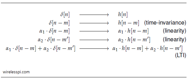
This leads to an input-output sequence as

During the above procedure, we have worked out the famous convolution equation that describes the output $r[n]$ for an input $s[n]$ to an LTI system with impulse response $h[n]$:

where the above sum is computed for each $n$ from $-\infty$ to $+\infty$. In this text, convolution operation is denoted by $*$ as
\begin{equation}\label{eqIntroductionConvolution2}
r[n] = s[n] * h[n]
\end{equation}

Note that
\begin{align}
s[n] * h[n] &= h[n] * s[n] \label{eqIntroductionConvolutionCommutative} \\
&= \sum \limits _{m = -\infty} ^{\infty} h[m] s[n-m] \nonumber
\end{align}

This can be verified by plugging $p = n-m$ in Eq \eqref{eqIntroductionConvolution1} which yields $m = n-p$ and hence $\sum _{p = -\infty} ^{\infty} s[n-p] h[p]$.

Convolution is a very logical and simple process but many DSP learners can find it confusing due to the way it is explained. As we did in transforming a signal, we will describe a conventional method and another more intuitive approach.

Conventional Method

Most textbooks after defining the convolution equation suggest its implementation through the following steps. For every individual time shift $n$,

[Flip] Arranging the equation as $r[n] = \sum _{m = -\infty} ^{\infty} s[m] h[-m+n]$, consider the impulse response as a function of variable $m$, flip $h[m]$ about $m = 0$ to obtain $h[-m]$.
[Shift] To obtain $h[-m+n]$ for time shift $n$, shift $h[-m]$ by $n$ units to the right for positive $n$ and left for negative $n$.
[Multiply] Point-wise multiply the sequence $s[m]$ by sequence $h[-m+n]$ to obtain a product sequence $s[m]\cdot h[-m+n]$.
[Sum] Sum all the values of the above product sequence to obtain the convolution output at time $n$.
[Repeat] Repeat the above steps for every possible value of $n$.

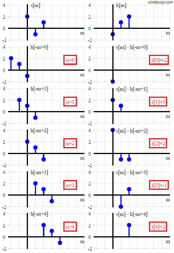
An example of convolution between two signals $s[n] = [2\hspace{1mm}-\hspace{-1mm}1\hspace{2mm} 1]$ and $h[n] = [-1\hspace{2mm} 1\hspace{2mm} 2]$ is shown in Figure below, where the result $r[n]$ is shown for each $n$.

Note a change in signal representation above. The actual signals $s[n]$ and $h[n]$ are a function of time index $n$ but the convolution equation denotes both of these signals with time index $m$. On the other hand, $n$ is used to represent the time shift of $h[-m]$ before multiplying it with $s[m]$ point-wise. The output $r[n]$ is a function of time index $n$, which was that shift applied to $h[-m]$.

Next, we turn to the more intuitive method where flipping a signal is not required.

Intuitive Method

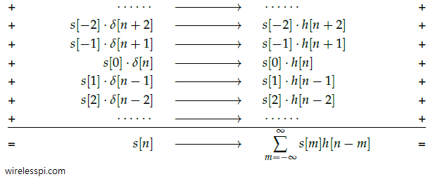
There is another method to understand convolution. In fact, it is built on the derivation of convolution equation Eq \eqref{eqIntroductionConvolution1}, i.e., find the output $r[n]$ as
\begin{align}
r[n] ~ &= ~ \cdots + \nonumber \\
&\qquad\quad s[-2]\cdot h[n+2] ~+ \nonumber \\
&\qquad\qquad \quad\quad\quad s[-1]\cdot h[n+1] ~+ \nonumber \\
&\qquad\qquad \qquad\qquad\quad \quad\quad \quad s[0]\cdot h[n] ~+ \nonumber \\
&\qquad\qquad \quad \qquad\qquad\qquad \quad \quad\quad~ s[1]\cdot h[n-1] ~+ \nonumber \\
&\qquad\qquad \qquad\qquad\qquad\qquad\qquad \quad\quad\quad \quad~ s[2]\cdot h[n-2] ~+ \nonumber \\
&\qquad\qquad \qquad\qquad\qquad\qquad\qquad\qquad\qquad\qquad\quad\quad\quad\quad \cdots \label{eqIntroductionConvolution3}
\end{align}
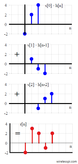
Let us solve the same example as in the above Figure, where $s[n] = [2\hspace{1mm}-~\hspace{-2mm}1\hspace{2mm} 1]$ and $h[n] = [-1\hspace{2mm} 1\hspace{2mm} 2]$. This is shown in Table below.

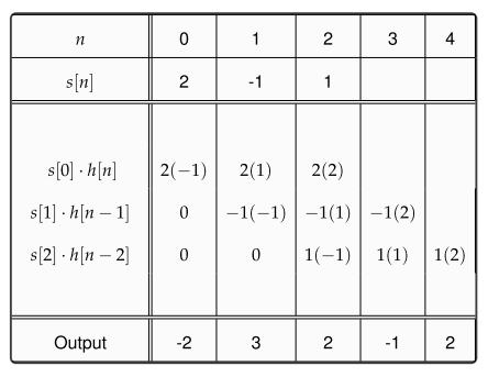
Such a method is illustrated in Figure below. From an implementation point of view, there is no difference between both methods.

Properties

Some important properties of convolution are as below.

[Length] From the above figures, we find that the length of the resultant signal $r[n]$ is $5$, when the lengths of both $s[n]$ and $h[n]$ are $3$ samples. This is a general rule:
\begin{equation}\label{eqIntroductionConvolutionLength}
\text{Length}\{r[n]\} = \text{Length}\{s[n]\} + \text{Length}\{h[n]\} – 1
\end{equation}
[First Sample] The first sample of the result is given by
\begin{equation}\label{eqIntroductionConvolutionFirstSample}
\text{First Sample}\{r[n]\} = \text{First Sample}\{s[n]\} + \text{First Sample}\{h[n]\}
\end{equation}

Since a single unit impulse $\delta [n]$ can only generate a single instance of impulse response $h[n]$, convolution of an impulse response by a unit impulse is the impulse response itself. This result is general and holds for any signal $s[n]$.
\begin{equation}\label{eqIntroductionUnitImpulseConvolution}
s[n] * \delta[n] = s[n]
\end{equation}

Significance of Complex Sinusoids

In a previous article about frequency response, we raised two questions about the frequency domain output for a unit impulse input and significance of complex sinusoids. To investigate these questions, let us excite an LTI system with a real impulse response $h[n]$ (i.e., $h_Q[n]=0$) by an input complex sinusoid $s[n]$ with
\begin{align*}
s_I[n]\: &= \cos 2\pi \frac{k}{N} n \\
s_Q [n] &= \sin 2\pi \frac{k}{N} n
\end{align*}

where $k/N$ is an arbitrary discrete frequency in the range $[-0.5,+0.5)$ as detailed in the post on discrete frequency. The output is given by convolution of the input and system impulse response as
\begin{align*}
r[n] &= s[n] * h[n] \\
&= \sum \limits _{m = 0} ^{N-1} s[m] h[n-m] \\
&= \sum \limits _{m = 0} ^{N-1} h[m] s[n-m ]
\end{align*}
where the last equality resulted from Eq \eqref{eqIntroductionConvolutionCommutative}. The $I$ and $Q$ components of the output are then expressed as
\begin{align*}
r_I[n] \: &= \sum \limits _{m = 0} ^{N-1} h[m] \cdot \cos 2\pi \frac{k}{N} (n-m) \\
r_Q [n] &= \sum \limits _{m = 0} ^{N-1} h[m] \cdot \sin 2\pi \frac{k}{N} (n-m)
\end{align*}

Expanding by identities $\cos (A-B)$ $=$ $\cos A \cos B$ $+$ $\sin A \sin B$ and $\sin$ $(A-B)$ $=$ $\sin A \cos B -$ $\cos A \sin B$,
\begin{align*}
r_I[n] \: &= \left\{ \sum \limits _{m = 0} ^{N-1} h[m] \cdot \cos 2\pi \frac{k}{N}m \right\} \cos 2\pi\frac{k}{N}n ~+ \\
& \hspace{1.4in}\left\{ \sum \limits _{m = 0} ^{N-1} h[m] \cdot \sin 2\pi \frac{k}{N}m \right\}\sin 2\pi\frac{k}{N}n \\
r_Q [n] &= – \left\{ \sum \limits _{m = 0} ^{N-1} h[m] \cdot \sin 2\pi \frac{k}{N}m \right\}\cos 2\pi\frac{k}{N}n ~+ \\
& \hspace{1.4in}\left\{ \sum \limits _{m = 0} ^{N-1} h[m] \cdot \cos 2\pi \frac{k}{N}m \right\} \sin 2\pi\frac{k}{N}n
\end{align*}

For a real $h[n]$ where $h[n] = h_I[n]$,
\begin{align*}
r_I[n] \: &= H_I[k] \cos 2\pi\frac{k}{N}n – H_Q[k] \sin 2\pi\frac{k}{N}n \\
r_Q [n] &= H_Q[k] \cos 2\pi\frac{k}{N}n + H_I[k] \sin 2\pi\frac{k}{N}n
\end{align*}

From the complex multiplication rule, the above equation can clearly be seen as a product between $H[k]$ and input complex sinusoid $s[n]$ as

A similar result holds for a complex impulse response. There can be a possibility of confusion regarding above Eq as how a time domain signal $s[n]$ can get multiplied with a frequency domain signal $H[k]$. This is not what the equation says. Actually, $s[n]$ is not an arbitrary input signal here. It is a specific complex sinusoid with discrete frequency $k/N$. All the equation says is that if given as an input, the same complex sinusoid appears at the output scaled by the system frequency response at discrete frequency $k/N$. Explicitly,
\begin{align}\label{eqIntroductionComplexSinusoidFreqResponse2}
r_I[n]\: &= |H[k]|\cos \left( 2\pi \frac{k}{N} n + \measuredangle H[k] \right)\\
r_Q [n] &= |H[k]| \sin \left( 2\pi \frac{k}{N} n + \measuredangle H[k] \right)
\end{align}

The significant conclusion from the above equation is that the output response of an LTI system to a complex sinusoid at its input is nothing but the same complex sinusoid at the same frequency but with different amplitude and phase. The following note answers the questions asked at the start of this article.

It can also be concluded from the above discussion that impulse response in time domain and frequency response in frequency domain are two equivalent descriptions of a system.

Convolution of Complex Signals

Convolution between a complex signal $s[n]$ input to a system with complex impulse response $h[n]$ can be understood through writing Eq \eqref{eqIntroductionConvolution1} in $IQ$ form. It is defined in a similar manner as
\begin{equation*}
r[n] = s[n] * h[n]
\end{equation*}
and can be decomposed as,
\begin{align*} \label{eqIntroductionComplexConvolution1}
r_I[n]\: &= s_I[n] * h_I[n] – s_Q[n] * h_Q[n] \\
r_Q[n] &= s_Q[n] * h_I[n] + s_I[n] * h_Q[n]
\end{align*}

The actual computations can be written as
\begin{align} \label{eqIntroductionComplexConvolution2}
r_I[n]\: &= \sum \limits _{m = -\infty} ^{\infty} s_I[m] h_I[n-m] – \sum \limits _{m = -\infty} ^{\infty} s_Q[m] h_Q[n-m] \\
r_Q[n] &= \sum \limits _{m = -\infty} ^{\infty} s_Q[m] h_I[n-m] + \sum \limits _{m = -\infty} ^{\infty} s_I[m] h_Q[n-m]
\end{align}

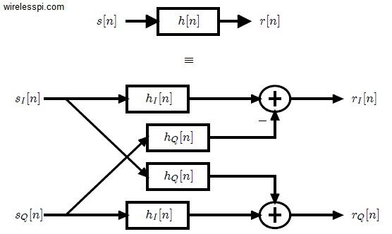
Due to the identity $\cos A \cos B – \sin A \sin B = \cos (A+B)$, a negative sign in $I$ expression indicates that phases of the two aligned-axes terms are actually adding together. Obviously, the identity applies in above equations only if magnitude can be extracted as common term, but the concept of phase-alignment still holds. Similarly, the identity $\sin A \cos B + \cos A \sin B = \sin (A+B)$ implies that phases of the two cross-axes terms are also adding together in $Q$ expression. Hence, a complex convolution can be described as a process that

• computes $4$ real convolutions: $I * I$, $Q * Q$, $Q * I$ and $I * Q$
• adds by phase aligning the $2$ aligned-axes convolutions ($I * I$ – $Q * Q$) to obtain the $I$ component
• adds the $2$ cross-axes convolutions ($Q * I$ + $I * Q$) to obtain the $Q$ component.

These computations are shown in Figure below.

Convolution and Frequency Domain

After understanding convolution both intuitively and mathematically, we want to see the interpretation of this process in frequency domain. Specifically, what is the DFT of $r[n] = s[n] * h[n]$? To answer this question, we want to apply the DFT definition to the result of Eq \eqref{eqIntroductionConvolution1}. However, we saw in the article about Discrete Fourier Transform that the way both time and frequency domain sequences are defined within a range $0 \le n, k \le N-1$, DFT works with circular shift which appears due to the inherent periodicity arising from sampling in frequency domain. That leads us to circular convolution.

Circular convolution between two signals, denoted by $\circledast$, is very similar to regular convolution except that the flipping and time shifts are circular as explained in the post about transforming a signal.
\begin{align}
r[n] &= s[n] \circledast h[n] \nonumber \\
&= \sum \limits _{m = 0} ^{N-1} s[m] h[(n-m) \:\text{mod}\: N] \label{eqIntroductionCircularConvolution}
\end{align}

Let us compute the DFT $R_k[n]$ of the resultant signal. We focus on real signals as the derivation for complex signals is similar. Since $r[n]$ is a real signal in our case, $r_I[n] = r[n]$ and $r_Q[n] = 0$, and the $I$ component in frequency domain $R_I[k]$ from the DFT definition can be expressed as
\begin{align*}
R_I[k] &= \sum \limits _{n=0} ^{N-1} r_I[n] \cos 2\pi\frac{k}{N}n \\
&= \sum \limits _{n=0} ^{N-1} \sum \limits _{m = 0} ^{N-1} s[m] h[(n-m) \:\text{mod}\: N] \cos 2\pi\frac{k}{N}n \\
&= \sum \limits _{n=0} ^{N-1} \sum \limits _{m = 0} ^{N-1} s[m] h[(n-m) \:\text{mod}\: N] \cos 2\pi\frac{k}{N} (n-m+m)
\end{align*}
Using the identities $\cos (A+B) = \cos A \cos B – \sin A \sin B$,
\begin{align*}
R_I[k] &= \sum \limits _{n=0} ^{N-1} \sum \limits _{m = 0} ^{N-1} s[m] h[(n-m) \:\text{mod}\: N] \cos 2\pi\frac{k}{N} (n-m) \cos 2\pi \frac{k}{N}m \\
&- \sum \limits _{n=0} ^{N-1} \sum \limits _{m = 0} ^{N-1} s[m] h[(n-m) \:\text{mod}\: N] \sin 2\pi\frac{k}{N} (n-m) \sin 2\pi \frac{k}{N}m
\end{align*}
The above equation can be rearranged as
\begin{align*}
R_I[k] &= \sum \limits _{m = 0} ^{N-1} s[m]\cos 2\pi \frac{k}{N}m \sum \limits _{n=0} ^{N-1} h[(n-m) \:\text{mod}\: N] \cos 2\pi\frac{k}{N} (n-m) \\
&- \sum \limits _{m = 0} ^{N-1} s[m] \sin 2\pi \frac{k}{N}m \sum \limits _{n=0} ^{N-1} h[(n-m) \:\text{mod}\: N] \sin 2\pi\frac{k}{N} (n-m)
\end{align*}
Since both $s[n]$ and $h[n]$ are real for the purpose of this derivation, and $\cos 2\pi \frac{k}{N} \{(n-n_0) \:\text{mod}\: N\}$ $=$ $\cos 2\pi \frac{k}{N} (n-n_0)$ while a similar identity holds for $\sin(\cdot)$,
\begin{align*}
R_I[k] &= S_I[k] \cdot H_I[k] – S_Q[k] \cdot H_Q[k]
\end{align*}

A similar computation for $Q$ component yields
\begin{align*}
R_Q[k] &= S_Q[k] \cdot H_I[k] + S_I[k] \cdot H_Q[k]
\end{align*}

Combining both equations above,
\begin{equation}\label{eqIntroductionConvolutionFreq}
R[k] = S[k] \cdot H[k]
\end{equation}
Therefore, we arrive at an extremely important result that is widely utilized in most DSP applications.

The inverse relation also holds. For discrete signals, multiplication of two time domain signals results in their circular convolution in frequency domain.
\begin{equation}\label{eqIntroductionMultiplicationConvolution}
s[n] \cdot h[n]~ \xrightarrow{\text{F}} ~ \frac{1}{N} \cdot S[k] \circledast H[k]
\end{equation}

The above finding is actually proved for regular convolution through continuous signals. Since we limit ourselves to discrete domain here, we deal with circular convolution and corresponding DFT only.