Some DFT Properties

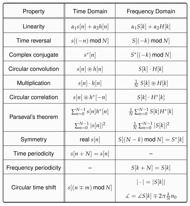
The purpose of this article is to summarize some useful DFT properties in a table. My favorite property is the beautiful symmetry depicted by continuous and discrete Fourier transforms.

However, if you feel that this particular content is not as descriptive as the other posts on this website are, you are right. As opposed to the rest of the content on the website, we do not intend to derive all the properties here. Instead, based on what we have learned, some important properties of the DFT are summarized in the table below with an expectation that the reader can derive themselves by following a similar methodology of plugging in the time domain expression in DFT definition.

Some of the examples are derived below.

Time Reversal and Complex Conjugation

---

From the time reversal and complex conjugation property,
\begin{equation}
s^*[(-n) \:\text{mod}\: N] ~\xrightarrow{\text{{F}}}~ S^*[k] \label{eqIntroductionTimeReversalComplexConjugation}
\end{equation}

To see why it is so, plug the expression $s^*[(-n) \:\text{mod}\: N]$ in DFT definition and let us call this DFT as $\widetilde{S}[k]$. Recall that in the complex conjugate, the $I$ part stays the same while $Q$ reverses in sign. Moreover, operation $\:\text{mod}\: N$ is implicitly assumed here even if not stated.
\begin{equation*}
\begin{aligned}
\widetilde{S}_I[k]\: &= \sum \limits _{n=0} ^{N-1} s_I [-n] \cos 2\pi\frac{k}{N}n – s_Q [-n] \sin 2\pi\frac{k}{N}n \\
\widetilde{S}_Q[k] &= -\sum \limits _{n=0} ^{N-1} s_Q[-n] \cos 2\pi\frac{ k}{N}n – s_I[-n] \sin 2\pi\frac{k}{N}n
\end{aligned}
\end{equation*}

Next, a change of variable from $n$ to $u$ is introduced such that $-n=u$. The limits remain the same due to the DFT input and output periodicity. Also, using the identities $- \cos A = \cos (-A)$ and $-\sin A = \sin (-A)$,
\begin{equation*}
\begin{aligned}
\widetilde{S}_I[k]\: &= \sum \limits _{u=0} ^{N-1} s_I [u] \cos 2\pi\frac{k}{N}u + s_Q [u] \sin 2\pi\frac{k}{N}u \\
\widetilde{S}_Q[k] &= -\sum \limits _{u=0} ^{N-1} s_Q[u] \cos 2\pi\frac{ k}{N}u + s_I[u] \sin 2\pi\frac{k}{N}u
\end{aligned}
\end{equation*}
which can be written as
\begin{equation*}
\begin{aligned}
\widetilde{S}_I[k]\: &= \sum \limits _{u=0} ^{N-1} s_I [u] \cos 2\pi\frac{k}{N}u + s_Q [u] \sin 2\pi\frac{k}{N}u \\
\widetilde{S}_Q[k] &= – \left[\sum \limits _{u=0} ^{N-1} s_Q[u] \cos 2\pi\frac{ k}{N}u – s_I[u] \sin 2\pi\frac{k}{N}u\right]
\end{aligned}
\end{equation*}

Comparing with the DFT definition, observe that the $I$ part is the same while the $Q$ part contains a negative sign. Thus,
\begin{equation}
\widetilde{S}[k] = S^*[k]
\end{equation}

In conclusion, the DFT of a time-reversed and complex conjugated signal is given by the complex conjugate of its DFT.

Conjugate Symmetry

---

In many of the figures encountered so far in this text, we observed some kind of symmetry in DFT outputs. More specifically, $I$ parts of the DFT had even symmetry while the $Q$ components were odd symmetric in many plots. Similarly, magnitude plots were even symmetric and phase plots had odd symmetry. This is true only for real input signals for which quadrature component is zero.

Such kind of symmetry is called conjugate symmetry defined as
\begin{equation}
S[N-k] = S^*[k]\label{eqIntroductionConjugateSymmetry}
\end{equation}
which implies
$$\begin{equation}
\begin{aligned}
S_I[N-k]\: &= S_I[k] \\
S_Q[N-k] &= -S_Q[k]
\end{aligned}
\end{equation}\label{eqIntroductionConjugateSymmetry1}$$
or
$$\begin{equation}
\begin{aligned}
|S [N-k]| &= |S[k]| \\
\measuredangle S [N-k] &= – \measuredangle S[k]
\end{aligned}
\end{equation}\label{eqIntroductionConjugateSymmetry2}$$
i.e., the $I$ component is even symmetric while the $Q$ part is odd symmetric. To see why real signals have a conjugate symmetric DFT, refer to the DFT definition. For a real signal, $s_Q[n]$ is zero and
$$\begin{equation}
\begin{aligned}
S_I[k]\: &= \sum \limits _{n=0} ^{N-1} s_I[n] \cos 2\pi\frac{k}{N}n \\
S_Q[k] &= – \sum \limits _{n=0} ^{N-1} s_I[n] \sin 2\pi\frac{k}{N}n
\end{aligned}
\end{equation}\label{eqIntroductionCSproof1}$$
Now $S[N-k]$ is defined as
\begin{align*}
S_I[N-k]\: &= \sum \limits _{n=0} ^{N-1} s_I[n] \cos 2\pi\frac{N-k}{N}n \\
S_Q[N-k] &= \sum \limits _{n=0} ^{N-1} – s_I[n] \sin 2\pi\frac{N-k}{N}n
\end{align*}
Using the identities $\cos (A-B) = \cos A \cos B + \sin A \sin B$, $\sin (A-B) = \sin A \cos B – \cos A \sin B$, $\cos 2 \pi n = 1$, $\sin 2\pi n = 0$, $\cos (-A) = \cos A$, and $\sin (-A) = -\sin A$, we get
$$\begin{equation}
\begin{aligned}
S_I[N-k]\: &= \sum \limits _{n=0} ^{N-1} s_I[n] \cos 2\pi\frac{k}{N}n \\
S_Q[N-k] &= \sum \limits _{n=0} ^{N-1} s_I[n] \sin 2\pi\frac{k}{N}n
\end{aligned}
\end{equation}\label{eqIntroductionCSproof2}$$
Eq \eqref{eqIntroductionCSproof1} and Eq \eqref{eqIntroductionCSproof2} satisfy the definition of conjugate symmetry in Eq \eqref{eqIntroductionConjugateSymmetry1} and the proof is complete.

---

As an example, observe an even symmetry in $I$ part of the DFT of a rectangular sequence and magnitude in this article. Similarly, an odd symmetry can be observed from the same figures for $Q$ part and phase, respectively.

Finally, observe that for real and even signals, the DFT is purely real and even, as $Q$ part is $0$. This can be verified from Eq \eqref{eqIntroductionCSproof1} because $Q$ term is then a product of an even signal and an odd signal $\sin 2\pi (k/N) n$ resulting in an odd signal. Half the values in an odd signal are the same as the other half but of opposite sign, and their sum is zero. Also, the $I$ part is a product of an even signal $s_I[n]$ and an even signal $\cos 2\pi (k/N)n$, generating an even output.

As an easy rule, whenever you see an even symmetric signal around $0$ whether in time or frequency domain, remember that its transform will be real and will only consist of an $I$ component. On the other hand, if the signal is not even symmetric whether in time or in frequency domain, its transform will contain a $Q$ component and hence will be complex in general.

Odd Symmetry

---

To use later, we now prove that a real and odd spectrum, i.e., with only an $I$ component that is an odd function of frequency, has an odd quadrature time component with a zero $I$ part. Referring to the iDFT definition and using the fact that $S_Q[k]$ is zero,
\begin{equation*}
\begin{aligned}
s_I[n]\: &= \frac{1}{N}\sum \limits _{k=-N/2} ^{N/2-1} S_I[k] \cos 2\pi\frac{k}{N}n \\
s_Q[n] &= \frac{1}{N}\sum \limits _{k=-N/2} ^{N/2-1} S_I[k] \sin 2\pi\frac{k}{N}n
\end{aligned}
\end{equation*}

Using the identity $\cos (-A) = \cos A$ in addition to $S_I[k]$ being odd, we can see that for a fixed $n$, half of the terms in $I$ part have one sign while the other half possess a reverse sign thus summing up to zero. On the other hand, $\sin (-A) = -\sin A$ and hence for a fixed $n$, when $S_I[k]$ reverses its sign, $\sin(\cdot)$ also reverses its sign, resulting in a nonzero $Q$ component. While $S_I[k]$ stays the same for all $n$, $\sin(\cdot)$ reverses its sign for half of the values of $n$ that leads to an odd response. We will apply this result during our discussion on band edge filters.

Parseval’s Relation

---

One of the most important properties of DFT we use over and over again is the Parseval’s relation that relates the energy of a signal in time domain with that in frequency domain.
\begin{equation*}
E_s = \sum _{n=0} ^{N-1} |s[n]|^2 = \frac{1}{N} \sum _{k=0} ^{N-1} |S[k]|^2
\end{equation*}
In words, energy of a signal in time domain is equal to its energy in frequency domain scaled by $1/N$. The intuitive reason for this scaling factor in frequency domain is that the DFT output for a complex sinusoid with amplitude $A_0$ is $A_0N$, an $N$ time magnification. The rest of the energy in frequency domain stays equal to the time domain, as demonstrated in sample rate conversion.