Time-Bandwidth Product (TBP) of a waveform is a foundational term frequently used in communications and radar community. However, I have never seen any book or online resource explain the core idea in an intuitive manner. Even though I understood the concepts of degrees of freedom and packing of resources in an $N$-dimensional space, I found it hard to come up with a visualization of time-bandwidth product in my head. This is what I set out to accomplish in this article.
Let us start with the term Bandwidth-Delay Product (BDP), a term frequently used in communication networks. We will shortly relate this to time-bandwidth product.
Bandwidth-Delay Product (BDP)
Assuming a binary modulation scheme and a rectangular pulse, each bit occupies a timespan of $T$ seconds. While the actual bandwidth of any finite duration signal is theoretically infinite, we adopt a certain definition for engineering purposes. In most cases, this is the width from the center to the first zero-crossing. As a consequence, the spectrum of this rectangular pulse is said to span $1/T$ Hz in frequency domain.
\begin{equation}\label{equation-rectangular-pulse-bandwidth}
\text{BW} \approx \frac{1}{T}
\end{equation}
A rectangular pulse and its spectrum are plotted in the figure below.

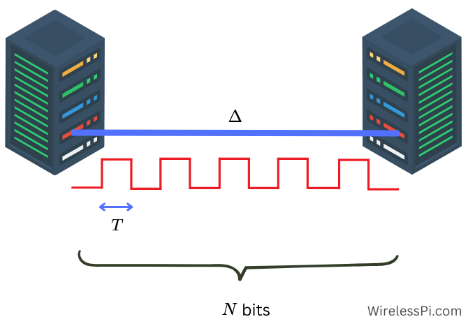
Now consider a simple one-way setup below which illustrates two network nodes connected through a link of length $L$ exchanging data at a rate such that the bit duration is $T$ seconds. Due to binary modulation, one can see the sequence of $+1$s and $-1$s going through the link.

If the signal propagates through the medium of length $L$ at a speed of $c$, then the delay it experiences (latency) while traveling from one node to another is given by $\Delta = L/c$. This comes from the relation time=distance/speed for an object moving at a constant speed. Considering the relation $B=1/T$ described in Eq (\ref{equation-rectangular-pulse-bandwidth}), the bandwidth-delay product is
\[
\begin{aligned}
\text{BDP} &= B\times \Delta \approx \frac{\Delta}{T} \\ \\
&= \frac{\text{Link length in time}}{\text{Bit duration}} = \text{No. of bits on the link}
\end{aligned}
\]
In words, the bandwidth-delay product turns out to be the number of bits $N$ going through the link at any time. This can also be seen from their units: seconds/(seconds/bit) which is the number of bits.
Looking at the above figure now, this framework generates a clear image of bandwidth-delay product for binary modulation in our heads: the number of bits “sitting” on the link at any given moment!
While we mostly limit ourselves to binary modulation in this article, multiple bits/symbol can be communicated during each interval $T$, which are known as symbols. For example, $2$ bits can be sent on one symbol if we have $4$ different amplitudes:
\[
\begin{aligned}
-3 \quad &\rightarrow \quad 00\\
-1 \quad &\rightarrow \quad 01\\
+1 \quad &\rightarrow \quad 10\\
+3 \quad &\rightarrow \quad 11
\end{aligned}
\]An interested reader can see how to pack more bits in one symbol for details.
So in reality, it is actually $N$ symbols “sitting” on the link which inherently translates into number of bits present at one moment.
\text{BDP} = \text{No. of symbols on the link}
\]
In the box below, I briefly describe this concept as used in TCP, which may be skipped if desired.
Keep in mind that instead of one-way delay, actual networks implementing the Transmission Control Protocol (TCP) use Round-Trip Time (RTT) for calculating this quantity because it translates into the amount of data required to fill the “pipe” before an acknowledgement from the other node can be received.
In other words, this is a transmission upper bound for the sender sliding window before it must stop and wait for an acknowledgement. Ideal networks operate with pipes that are always full.
As a simple example, for a $10$ Mbps link with RTT of $100$ ms, we get
\[
\text{BDP} = 10\times 10^6\times 100\times 10^{-3} = 1~\text{Mb} = 125~\text{kB}
\]
as the maximum amount of data that can be in flight during any given moment.
With this understanding in place, we now move towards the time-bandwidth product.
Time-Bandwidth Product (TBP)
You would have noticed that time-bandwidth product is, in some way, similar to bandwidth-delay product, except that here we have time duration of a pulse instead of delay.
\[
\begin{aligned}
\text{Bandwidth} \qquad &\leftrightarrow \qquad \text{Bandwidth} \\
\text{Delay}\qquad &\leftrightarrow \qquad \text{Time}
\end{aligned}
\]
However, delay is a form of time too. Therefore, we conclude that time-bandwidth product tells us about $N$ units of something. What is it?
Let us start with the rectangular pulse described before. Using Eq (\ref{equation-rectangular-pulse-bandwidth}), we can write its time-bandwidth product as
\[
\text{TBP} = T\times B ~\approx~ T\times\frac{1}{T} = 1
\]
From the viewpoint of TBP, the above values implies that there is only one parameter that can be controlled in this pulse shape, which obviously is the pulse duration $T$. Regardless of how long the time $T$ is, the time-bandwidth product is always $1$. This is because there is no variation in the pulse and hence bandwidth itself is dependent on its duration.
Let us now break the link between pulse duration and bandwidth.
Amplitude
What happens when we switch the amplitude between two or more values at fixed intervals within the pulse duration? Consider an amplitude modulated pulse $s_n(t)$ of duration $\tau$ as
\[
s_n(t) = A_n, \qquad 0 \le t \le \tau
\]
where $A_n = \pm 1$ at time $n$. From here, $N$ such amplitude modulated chips can be joined together to form a single waveform of duration $T$ as before. This is drawn in the figure below where the amplitude of the whole signal at the bottom is not constant anymore. While having the same duration $T$, the new waveform exhibits a sequence of $+1$s and $-1$s (note that the variation does not have to appear in each symbol interval due to random data).

Mathematically, we can write this cumulative signal as
\[
s(t) = \sum _{n=0}^{N-1} s_n(t-n\tau)
\]
which basically places the $n$-th signal $s_n(t)$ at time $n$. This implies that the total timespan of the waveform can be written as $T = N\tau$. In other words, we have a total of $N$ basic amplitude modulated units as
\[
N = \frac{T}{\tau}
\]
For example, the figure above shows $N=13$ units. In the spirit of Eq (\ref{equation-rectangular-pulse-bandwidth}), the bandwidth of this signal is now given by
\[
B \approx \frac{1}{\tau}
\]
As a consequence, the time-bandwidth product can be written as
\begin{equation}\label{equation-time-bandwidth-product-amplitude}
\text{TBP} = T\times B = T \times \frac{1}{\tau} = N
\end{equation}
These $N$ smaller pulses can be controlled by assigning them different amplitudes completely independent of each other, just like those $N$ symbols “sitting” on the link at any given moment in bandwidth-delay product.
As compared to the rectangular pulse where the product was only $1$, we now have $N$ as the TBP here. Now let us write the carrier modulated wave as
\[
s_n(t) = A_n\cos \left(2\pi F_ct + \phi\right)
\]
where $F_c$ is the carrier frequency and $\phi$ is an arbitrary phase. When such a signal is sampled at a rate of $F_s$ samples/second after downconversion, the Nyquist sampling theorem dictates the minimum sample rate $F_s$ as
\[
\begin{aligned}
F_s &= 2B \qquad \text{For real signals}\\
F_s &= B \qquad ~~\text{For complex signals}
\end{aligned}
\]
Going with the complex sampling scenario, the total number of samples obtained within the waveform of duration $T$ is
\[
\text{seconds}\cdot\text{samples/second} = T\times F_s = T\times B = N
\]
where we have used Eq (\ref{equation-time-bandwidth-product-amplitude}) for arriving at the last step. We conclude that in discrete domain, these $N$ samples define a complex $N$-dimensional space.
Phase
Amplitude is not the only knob we can turn in obtaining a higher time-bandwidth product. In communications and radar applications, phase and frequency can also be utilized for this purpose.
Similar to the amplitude, a phase modulated subpulse can be written as
\[
s_n(t) = A\cos \left(2\pi F_ct + \phi_n\right)
\]
where now the amplitude $A$ is constant while the phase $\phi_n$ varies at time $n$. The figure below plots a random sequence of phases, either $0^\circ$ or $180^\circ$ at each instant. While here it is essentially amplitude modulation ($+1$s and $-1$s) riding on a carrier wave, it can take more phases from a higher-order modulation.

Just like the previous case, the time-bandwidth product is still given by $N$ that can be conveniently obtained by sampling the signal at a rate of $1$ sample/symbol.
We now turn our attention towards frequency modulation.
Frequency
As far as time-bandwidth product in a frequency modulated waveform is concerned, I describe a simple example of a stepped-frequency signal divided into three parts, corresponding to frequencies $F_1$, $2F_1$ and $3F_1$, i.e., they are integer multiples of a fundamental frequency $F_1$. Mathematically,
\[
s_n(t) = A\cos \left(2\pi F_nt + \phi\right)
\]
The cumulative signal is plotted in the figure below. The yellow boxes represent samples taken at regular intervals, as we shortly see.

Notice the first sinusoid spanning one cycle within the first subpulse, the second sinusoid completing two cycles in the second interval while the third sinusoid spanning three cycles within the third subpulse. This is why we can observe discontinuities at their boundaries. Since these sinusoids are orthogonal to each other, i.e., they do not interfere with each other, we have time-bandwidth product in a similar manner as amplitude and phase.
A more practical case is that of a chirp, which is a similar waveform as above, but with a continuously varying frequency $\mu t + F_0$ (see LoRa PHY for more details on a chirp), also known as a Linear Frequency Modulated (LFM) signal. This is drawn in the figure below where the frequency can be seen as going from an initial frequency $F_1$ to a final frequency $F_3$ in a continuous manner.

The bandwidth of this signal is the range of frequencies contained within it, i.e., $B = F_3-F_1 = \Delta_F$. The time-bandwidth product is now
\[
\text{TBP} = T\times \Delta_F
\]
In a discrete-time system, the minimum sample rate $F_s=1/T_s$ for complex signals is equal to $B$, as described before. Since $B$ is $\Delta_F$ in this case and $T=NT_s$ for $N$ samples within the waveform duration, we get
\[
\text{TBP} = NT_s\times F_s = N
\]
which again gives us $N$ independent components for a linear chirp.
Significance of Time-Bandwidth Product
As we saw in amplitude, phase and frequency examples above, time-bandwidth product, or $BT$, reflects the number of independent components present in any waveform of duration $T$. These independent components are known as Degrees of Freedom (DoF). This basically tells us the number of complex numbers $N$ required to represent that signal of duration $T$. This is very similar to representing a point in 3D space, the only difference being the availability of $N$ dimensions instead of just $3$. In this context, it can be seen as the “information capacity” of the waveform.
If we attempt to characterize this signal with a number of samples less than $N$, it will result in aliasing. The signal loses degrees of freedom because higher-frequency components are “folded” onto lower frequencies, thus fundamentally altering the signal.
We can say that sampling “locks” the degrees of freedom into a discrete set. We now turn towards its significance in communications and radar applications.
Communications
In general, a signal that is compact in time domain is wide in frequency domain and vice versa. Therefore, a short pulse with less Inter-Symbol Interference (ISI) will have a wide spectrum. On the other hand, making it compact in frequency domain produces a time domain pulse with long sidelobes.
- For some signals (e.g., a rectangular pulse, a sinusoidal signal, etc.), the time-bandwidth product is small and it has less number of degrees of freedom. A small time-bandwidth product is useful in some applications. For example, the GSM standard used a Gaussian Minimum-Shift Keyed (GMSK) pulse with $BT=0.3$.
- This was chosen to make the spectrum more compact, thus fitting the signals within $200$ kHz narrow channels.
- This value also introduces some ISI because each pulse is spread over approximately 3 bit periods due to the particular Gaussian response, but most of the power spectrum remains within the designated bandwidth.
Therefore, such a choice provides a compact spectrum while also minimizing ISI, thus striking a nice tradeoff. A GMSK pulse with different time-bandwidth products, including the GSM value of $0.3$, is plotted in the figure below.
- This gives us a hint that time-bandwidth product is a measure of how well the available bandwidth is utilized for communications. Since we saw $N$ degrees of freedom in the case of amplitude, phase and frequency modulation in the last section, we can transmit $N$ symbols (or bits in case of binary modulation) in each such waveform. Given the same bit rate, this proves useful in narrowband interference mitigation, combating impulse noise and channel sounding applications.
Moreover, spread spectrum systems like Direct Sequence Spread Spectrum (DSSS) and Frequency Hopping Spread Spectrum (FHSS) use high time-bandwidth product to resist jamming, enable low probability of intercept and provide multiple access (as in some 2G and 3G wireless standards) because the energy is spread thinly over a wide bandwidth.
The emerging field of Integrated Sensing and Communication (ISAC) has made the time-bandwidth product of a waveform even more relevant.

Radar
Let us take an example of radar and see how a larger time-bandwidth product helps in better range resolution with the same pulse energy.
When a rectangular pulse is correlated with itself, the result is a triangular pulse which naturally has a gradual rolloff towards zero. This is because time-bandwidth product of a rectangular pulse is small. If this pulse returns as an echo after encountering a target, as long as there is some overlap between the two echoes, the targets cannot be distinguished from each other. The boundary at which this occurs is the point at which the two echoes are barely touching each other, i.e., the pulse width $T$. Converting from time to distance, the range resolution $\Delta_R$ can be written as
\begin{equation}\label{equation-radar-range-resolution}
\Delta_R = \frac{cT}{2}
\end{equation}
where the factor of $2$ comes due to signal transmission and return paths. From this expression, we can observe that a shorter pulse means finer resolution for the radar to distinguish close targets, while a longer pulse blurs nearby echoes into one. But a shorter pulse has less energy for the same peak amplitude, thus reducing the SNR and degrading the detection performance.
On the other hand, when a waveform with a large time-bandwidth product is correlated with itself, this results in pulse compression. The figure below plots the normalized correlation outputs of a chirp for two time-bandwidth products: $BT=10$ and $BT=50$. Also shown for comparison is the output for a rectangular pulse, which is a triangular pulse depicted as an orange line.

The benefit of pulse compression is evident if we determine the first zero-crossing of this sinc-like signal. Why zero-crossing? Because it dictates the range resolution of the pulsed radar. For this purpose, recall from the Fourier Transform that as a general rule, the first zero-crossing of a sinc signal in one domain is given by the inverse width of the rectangle in the other domain. Since the chirp contains all the frequencies within $B$ similar to a rectangular signal, we get
\[
\text{First zero-crossing} = \frac{1}{B}
\]
Notice from the above figure that with $T=1$, this first zero-crossing is at approximately $1/10=0.1$ for $B=10$ in the top plot and $1/50=0.02$ for $B=50$ in the bottom plot. Two return echoes can be separated as long as they arrive with at least this much delay at the Rx. Therefore, we can intuitively write the range resolution as
\begin{equation}\label{equation-radar-range-resolution-lfm}
\Delta R = \frac{c}{2}\cdot \text{First zero-crossing} = \frac{c}{2B}
\end{equation}
Compare this expression with the range resolution of the simple pulse in Eq (\ref{equation-radar-range-resolution}), i.e., $cT/2$. Since the pulse duration $T$ is the same for both a simple and an LFM pulse, they will exhibit the same peak power and output SNR at the correlation (or matched filter) output. But the improvement in range resolution can be written as
\text{Gain} = \left.\frac{cT}{2}\middle/\frac{c}{2B}\right. = BT
\]
In words, the LFM pulse achieves a processing gain equal to the time-bandwidth product as compared to a rectangular pulse of the same duration. In an external environment, this results in improved range resolution where one target can be distinguished from another target with a small difference in range. For a length-13 Barker sequence, this improved range resolution is shown in the figure below.

The above figure also demonstrates that in an indoor environment, a signal with high time-bandwidth product provides high multipath resolution where the radar can resolve individual paths, allowing the receiver to distinguish the direct signal from reflections for precision ranging (e.g., for centimeter-level accuracy in indoor positioning systems).
Conclusion
In technical terms, the idea of time-bandwidth product is as follows. Given a band limited waveform limited to $B$ Hz observed for total time $T$, we can uniquely describe that waveform with $N$ samples in time, thanks to the sampling theorem. Going into the frequency domain through the Discrete Fourier Transform (DFT), we can also describe the same waveform with $N$ samples in frequency. Ultimately, these are two ways to describe a single finite-energy waveform with $N$ complex degrees of freedom, meaning that one waveform resides in an $N$-dimensional complex vector space!
Generalizing this principle, the waveform can be represented with any orthonormal basis that spans the same space, such as complex Walsh codes. No matter which case we take, each of those $N$ samples can come from a Quadrature Amplitude Modulation (QAM) symbol on a complex plane.
Special thanks to Dan Boschen (the DSP Coach) for a discussion on $N$ complex degrees of freedom in time and frequency domains.