The most commonly used filter in DSP applications is a moving average filter. In today’s world with extremely fast clock speeds of the microprocessors, it seems strange that an application would require simple operations. But that is exactly the case with most applications in embedded systems that run on limited battery power and consequently host small microcontrollers. For noise reduction, it can be implemented with a few adders and delay elements. For lowpass filtering, the excellent frequency domain response and substantial suppression of stopband sidelobes are less important than having a basic filtering functionality, which is where a moving average filter is most helpful. Furthermore, there are smarter ways for this moving average implementation such as Cascaded Integrator Comb (CIC) filters that are widely used in digital radio frontends and other sample rate conversion applications.
As the name implies, a length-$M$ moving average filter averages $M$ input signal samples to generate one output sample. Mathematically, it can be written as
\begin{align*}
r[n] &= \frac{1}{M} \sum \limits_{m=0}^{M-1} s[n-m]\\
&= \sum \limits_{m=0}^{M-1} \frac{1}{M} \cdot s[n-m] \\
&= \sum \limits_{m=0}^{M-1} h[m] s[n-m]
\end{align*}
where as usual, $s[n]$ is the input signal, $r[n]$ is the system output and $h[n]$ is the impulse response of the moving average filter given by
\begin{equation*}
h[n] = \frac{1}{M}, \qquad n = 0,1,\cdots,M-1
\end{equation*}
The above discussion leads us to the following observations.
Impulse response From the above equation, the impulse response of a moving average filter can be seen a rectangular pulse which is drawn in Figure below. In terms of filtering, a constant amplitude implies that it treats all input samples with equal significance. This results in a smoothing operation of a noisy input [1].

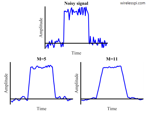
To see an example of noise reduction in time domain, consider a pulse in Figure below in which random noise is added. Observe that a longer filter performs a better smoothing action on the input signal. However, the longer length translates into wider edges during the transition.
Magnitude response As a consequence of its flat impulse response, the frequency response of a moving average filter is the same as the frequency response of a rectangular pulse, i.e., a sinc signal. The magnitude response of such a filter is drawn in the figure below. It is far from the brickwall response of an ideal lowpass filter but the magnitude response still has a shape that passes low frequencies with some distortion and attenuates high frequencies to some extent.
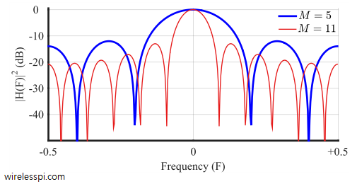
Due to this insufficient suppression of sidelobes, it is probably the worst lowpass filter one can design. On the other hand, as described earlier, its simplicity of implementation makes it useful for many applications requiring high sample rates including wireless communication systems. In such conditions, a cascade of moving average filters is implemented in series such that each subsequent filter inflicts more suppression to higher frequencies of the input signal.
Due to the inverse relationship between time and frequency domains, a longer filter in time domain produces a narrower frequency response. This can be observed in the impulse and frequency response for filter lengths $M=5$ and $M=11$.
Phase response As described in the article on FIR filters, a moving average filter generates a delay of $0.5(M-1)$ samples (for odd $M$) in the output signal as compared to an input signal. This delay manifests itself in the form of a linear phase in frequency domain.
Convolution Notice from above equations that the filter output is a convolution of the input signal with the impulse response of the moving average filter, a rectangular pulse.
References
[1] The Scientist and Engineer’s Guide to Digital Signal Processing (1st Edition), California Technical Pub., 1997.

