As we saw here, a signal is any measurable quantity that varies with time (or some other independent variable). Classification of continuous-time and discrete-time signals deals with the type of independent variable. If the signal amplitude is defined for every possible value of time, the signal is called a continuous-time signal. However, if the signal takes values at specific instances of time but not anywhere else, it is called a discrete-time signal. Basically, a discrete-time signal is just a sequence of numbers.
Consider a football (soccer) player participating in a 20-match tournament. Suppose that his running speed is recorded at each instant of time in the 90-minute duration of a particular match and plotted against time. The result shown in Figure below is clearly a continuous-time signal.

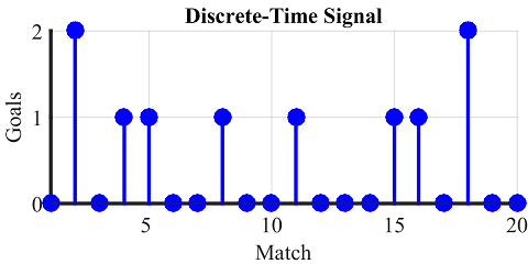
On the other hand, Figure below shows the number of goals he scored during those 20 matches, which is defined only for each match and not in between. Hence, it is a discrete-time signal.

Discrete-time signals usually arise in two ways:
- Inherently discrete-time: By recording the number of events over finite time periods. For example, number of trees cut every year in a city for housing and development projects.
- Conversion from continuous-time to discrete-time: By acquiring the values of a continuous-time signal at fixed time instants. This process is called sampling and is discussed in detail in another article. For example, the actual temperature outside varies continuously throughout the day, but weather stations log the data after specific intervals, say every 30 minutes.
Mathematically, we represent a continuous-time signal as $s(t)$ and a discrete-time signal as $s[n]$, where $t$ is a real number while $n$ is an integer. For example, a discrete-time signal $s[n] = 3n^2$ can be plotted by finding $s[n]$ for various values of $n$. Each member $s[n]$ of a discrete-time signal is called a sample.
\begin{align*}
n = -5 \quad \rightarrow \quad s[n] &= 75 \nonumber \\
n = -4 \quad \rightarrow \quad s[n] &= 48 \nonumber \\
n = -3 \quad \rightarrow \quad s[n] &= 27 \nonumber \\
n = -2 \quad \rightarrow \quad s[n] &= 12 \nonumber \\
n = -1 \quad \rightarrow \quad s[n] &= 3 \nonumber \\
n = 0 \quad \rightarrow \quad s[n] &= 0 \nonumber \\
n = +1 \quad \rightarrow \quad s[n] &= 3 \nonumber \\
n = +2 \quad \rightarrow \quad s[n] &= 12 \nonumber \\
n = +3 \quad \rightarrow \quad s[n] &= 27 \nonumber \\
n = +4 \quad \rightarrow \quad s[n] &= 48 \nonumber \\
n = +5 \quad \rightarrow \quad s[n] &= 75 \nonumber
\end{align*}
Plotting each value of $s[n]$ against every $n$ is then straightforward as shown in Figure below.

Another way of representing a discrete-time signal is in the form of a sequence with an underline indicating the time origin ($n=0$), such as
\begin{equation*}
s[n] = \{…,75, 48, 27, 12, 3, 0, 3, 12, 27, 48, 75, … \}
\end{equation*}
Finally, it is incorrect to assume that a discrete-time signal is zero between two values of $n$. It is simply not defined for non-integer values.
In electrical engineering, the time-varying quantity is usually voltage (or sometimes current). Therefore, when we work with a signal, just think of it as a voltage changing over time. After we convert this signal from continuous-time to discrete-time, it becomes a sequence of numbers.
Unit Impulse and Unit Step Signals
Some basic signals play an important role in discrete-time signal processing. We discuss two of them below.
- A unit impulse is a signal that is 0 everywhere, except at $n=0$, where its value is 1. Mathematically, it is denoted as $\delta[n]$ and defined as
\begin{equation}
\delta[n] = \left\{ \begin{array}{l}
1, \quad n = 0 \\
0, \quad n \neq 0 \\
\end{array} \right.
\end{equation}
The unit impulse signal is shown in Figure below. - A unit step signal is 0 for past ($n<0$) values, while 1 for present ($n=0$) and future ($n>0$) values. To be precise, it is denoted as $u[n]$ and defined as
\begin{equation}
u[n] = \left\{ \begin{array}{l}
1, \quad n \geq 0 \\
0, \quad n < 0 \\ \end{array} \right. \end{equation} The unit step signal is shown in Figure below.


Energy of a Signal
Plotting a discrete-time signal or writing it as a sequence of numbers seems good enough, but then how do we make a comparison between two signals? For example, in the case of soccer player above, we need to know how this player stands against other players participating in the tournament. It therefore seems that we should devise some measure of “strength” or “size” of a signal.
One simple method can be just adding all the values on the amplitude axis, which is our target dependent variable. So from the figure depicting player 1 goals, our player has a total number of 10 goals in the tournament. Now we can easily compare his performance with others, provided that the signal always stays positive.
Imagine another footballer who is so “energetic” that he just cannot resist possessing the ball during the game and sometimes even scores own goals, as shown in Figure below. From his team’s point of view, his net total by adding all goals is just 7. However, from an energy perspective in the field, he is much different than player 1 before.

Therefore, a simple addition does not work for signals that assume both positive and negative values, such as a voltage varying with time because addition of both positive and negative values cancels and diminishes the calculated signal strength. This suggests that strength of a signal can be measured by taking the absolute value of the signal and then adding all the values. Or square of the absolute value, or the fourth power of the absolute value, and so on. Due to its mathematical tractability (an exciting must-have for communication theorists), square of the absolute value is the preferred choice.
In light of the above, the energy of a discrete-time signal is defined as
\begin{align}
E_s &= \cdots + |s[-2]|^2 + |s[-1]|^2 + |s[0]|^2 + |s[1]|^2 + |s[2]|^2 + \cdots \nonumber \\
&= \sum \limits _n |s[n]|^2
\end{align}
where the term $\sum \limits _n$ denotes summation over all values of $n$.
As an example, signal energy in the figure depicting player 1 goals is
\begin{equation*}
E_{P1} = 2^2 + 1^2 + 1^2 + 1^2 + 1^2 + 1^2 + 1^2 + 2^2 = 14
\end{equation*}
and for the figure showing player 2 goals, it is
\begin{align*}
E_{P2} &= 2^2 + -1^2 + 1^2 + 1^2 + -1^2 + 1^2 + … \\
&\quad -1^2 + 2^2 + 1^2 + 1^2 + 2^2 + -1^2 = 21
\end{align*}
Using such a definition, the difference between the energy levels of the two players is truly reflected.
Similarly, energy in the quadratic signal above is infinite as the signal values extend from $-\infty$ to $+\infty$.
Even and Odd Signals
Some signals have specific properties which make analysis and computations simpler for us later. For example, a signal is called even (or symmetric) if
\begin{equation}
s[-n] = s[n] \quad \text{or} \quad s(-t) = s(t)
\end{equation}
Flipping an even signal around amplitude axis results in the same signal. An example of an even signal is $s(t) = \cos(2\pi f_0 t)$ shown in the left Figure below. The quadratic signal $s[n] = n^2$ illustrated before is also an even signal.

On the other hand, a signal is called odd (or antisymmetric) if
\begin{equation}
s[-n] = -s[n] \quad \text{or} \quad s(-t) = -s(t)
\end{equation}
An odd signal has symmetry around the origin. An example of an odd signal is $s(t) = \sin(2\pi f_0 t)$ drawn in the right Figure above, as well as $s[n] = -n$.
Periodic and Aperiodic Signals
A signal is periodic if it repeats itself after a certain period $N$.
\begin{equation}
s[n\pm N] = s[n] \quad \text{for all} ~n
\end{equation}
Both $s[n] = \cos[2\pi f_0 n]$ and $s[n] = \sin[2\pi f_0 n]$ are examples of periodic signals if $f_0$ is a rational number.
If a signal does not repeat itself forever, there is no value of $N$ that satisfies the above periodicity equation. Such a signal is known as aperiodic, an example of which is a unit step signal $u[n]$ and most other signals encountered in these articles.
An example each of a periodic and an aperiodic signal is shown in Figure below.