I have described in detail the story of the Kalman Filter (KF) in a previous article using intuitive arguments. The Kalman filter is applicable to linear models. Today we will learn about extending the Kalman filter to non-linear scenarios through an extended Kalman filter.
Numerous applications today require estimating the range, velocity, and acceleration of objects moving along a straight path. It could be an airplane within the scope of a traditional radar or an autonomous vehicle cruising down a road in an ever-connected society. And who knows, perhaps the superhumans of the next century will engage in futuristic play with bullets as toys.

We start with a system model and explain where the non-linearity comes from.
System Model
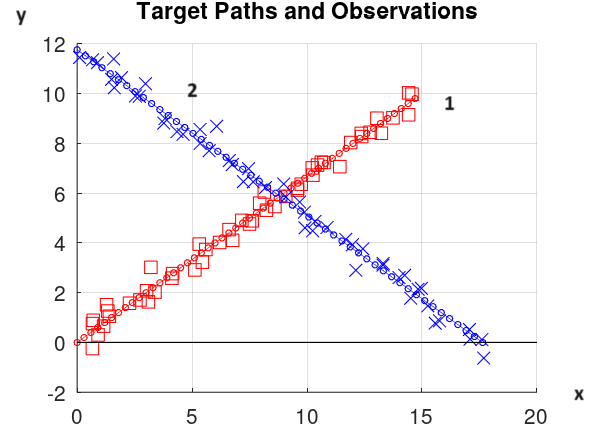
Two objects traveling in different directions in a 2-D motion are shown in the figure below. The job of the filter is to estimate four variables here: x-position, y-position, x-velocity and y-velocity of a given target.

State Transition
The state of an object moving in a straight line with a constant velocity changes only slightly from the previous moment. The actual position $x_n$ can be expressed as
$$
\begin{equation}
\begin{aligned}
x_n &= x_{n-1}+\Delta \cdot v_{x,n-1} + \text{process noise}\\
y_n &= y_{n-1}+\Delta \cdot v_{y,n-1} + \text{process noise}\\
v_{x,n} &= v_{x,n-1} + \text{process noise}\\
v_{y,n} &= v_{y,n-1} + \text{process noise}
\end{aligned}
\end{equation}\label{equation-extended-kalman-filter-model}
$$
where
- $n$ is the current time index,
- $x_{n-1}$ and $y_{n-1}$ are the x-position and y-position at time $n-1$, respectively,
- $v_{x,n}$ and $v_{y,n}$ are the velocities along the x-axis and y-axis, respectively,
- $\Delta$ is the time duration between one observation and the next (according to the rate at which the object is being probed), and
- process noise includes all the inaccuracies not accounted for in the model.
In matrix notation, this can be written as
\[
\begin{bmatrix}
x_n \\ y_n \\ v_{x,n} \\ v_{y,n}
\end{bmatrix}
= \begin{bmatrix}
1 & 0 & \Delta & 0\\
0 & 1 & 0 & \Delta\\
0 & 0 & 1 & 0 \\
0 & 0 & 0 & 1
\end{bmatrix}
\begin{bmatrix}
x_{n-1}\\ y_{n-1} \\ v_{x,n-1} \\ v_{y,n-1}
\end{bmatrix} + \text{process noise}
\]
Here, the state vector of this dynamic motion is given by
\[
\mathbf{x} = \begin{bmatrix}
x_n \\ y_n \\ v_{x,n} \\ v_{y,n}
\end{bmatrix}
\]
Also, the state transition matrix can be seen from the above expression as
\[
\mathbf{F} = \begin{bmatrix}
1 & 0 & \Delta & 0\\
0 & 1 & 0 & \Delta\\
0 & 0 & 1 & 0 \\
0 & 0 & 0 & 1
\end{bmatrix}
\]
Clearly, the system is linear in terms of the state transition matrix $\mathbf{F}$. In some situations, it is possible that the state transition matrix is non-linear. In that case, we can represent the above relation as
\[
\mathbf{x_n} = f(\mathbf{x_{n-1}}) + \text{noise}
\]
where $f(\cdot)$ captures the non-linear association between the state vector and the dynamic model. Let us go to the relationship between measurements and the state vector now.
Measurements
A tracking system needs not have the state vector measurements directly available. Instead, it might get a set of measurements related to the system variables. For example, a radar can gather information about the range $r_n$ through a back-and-forth time delay measurement, velocity or range rate $\dot r_n$ through Doppler shift of the received signal and azimuth angle $\theta_n$ from multiple antennas.
Now the range in terms of x-position $x_n$ and y-position $y_n$ can be expressed as
\begin{equation}\label{equation-extended-kalman-filter-range}
r_n = \sqrt{x_n^2+y_n^2} +\text{noise}
\end{equation}
On the other hand, the range rate is related to these position measurements by taking its derivative.
$$\begin{equation}
\begin{aligned}
\dot r_n &= \frac{1}{2}\left(x_n^2+y_n^2\right)^{-1/2}\left(2x_n\dot x_n + 2y_n \dot y_n\right) + \text{noise}\\
&= \frac{x_n\dot x_n + y_n \dot y_n}{\sqrt{x_n^2+y_n^2}} + \text{noise}
\end{aligned}
\end{equation}\label{equation-extended-kalman-filter-range-rate}$$
Finally, the azimuth angle $\theta_n$ is linked to the x-axis and y-axis positions as
\begin{equation}\label{equation-extended-kalman-filter-angle}
\theta_n = \tan^{-1}\left(\frac{y_n}{x_n}\right) + \text{noise}
\end{equation}
There is no linear relation between the measurements $\{r_n$, $\dot r_n$, $\theta_n\}$ and the state variables $\mathbf{x}$. Therefore, we cannot write the measurements as in the case of Kalman filter.
\[
\mathbf{z_n} = \begin{bmatrix}
r_n \\ \dot r_n \\ \theta_{n}
\end{bmatrix} \neq \mathbf{Hx_n}+ \text{noise}
\]
Instead, we define this relation as
\[
\mathbf{z_n} = h\left(\mathbf{x_n}\right)+ \text{noise}
\]
where the non-linearity $h(\cdot)$ can be observed in the previous equations. We will now see that how an extended Kalman filter can be applied in this situation.
Extended Kalman Filter
Recall that the Kalman filter algorithm is given in the figure below.

The Extended Kalman Filter is derived through applying the most common technique for dealing with non-linearities: we expand the non-linear function in a Taylor series around a particular point by making use of a Jacobian matrix and ignore the higher-order terms. This point differs depending on whether the non-linearity arises in the state transition matrix or the measurement matrix.
In the given scenario, the Jacobian matrix is defined as
\begin{equation}\label{equation-extended-kalman-filter-jacobian}
\mathbf{H} = \frac{\partial h}{\partial x}\bigg|_{x=\mathbf{x_{n,\text{prior}}}} = \left.\begin{bmatrix}
\frac{\partial h_1}{\partial x_1} & \frac{\partial h_1}{\partial x_2}& \frac{\partial h_1}{\partial x_3} & \frac{\partial h_1}{\partial x_4}\\
\frac{\partial h_2}{\partial x_1} & \frac{\partial h_2}{\partial x_2}& \frac{\partial h_2}{\partial x_3} & \frac{\partial h_2}{\partial x_4}\\
\frac{\partial h_3}{\partial x_1} & \frac{\partial h_3}{\partial x_2}& \frac{\partial h_3}{\partial x_3} & \frac{\partial h_3}{\partial x_4}
\end{bmatrix}\right|_{x=\mathbf{x_{n,\text{prior}}}}
\end{equation}
While the above expression looks complicated, it can be applied to the linear motion example under consideration for clarity.
Range
From Eq (\ref{equation-extended-kalman-filter-range}), $r_n$ is equal to $\sqrt{x_n^2+y_n^2}$. Therefore, we have
\[
\frac{\partial h_1}{\partial x_1} = \frac{\partial r_n}{\partial x_n} = \frac{\partial}{\partial x_n} \left(x_n^2+y_n^2\right)^{1/2} = \frac{x_n}{\sqrt{x_n^2+y_n^2}}
\]
Similarly,
\[
\frac{\partial h_1}{\partial x_2} = \frac{\partial r_n}{\partial y_n} = \frac{y_n}{\sqrt{x_n^2+y_n^2}}
\]
Moreover,
\[
\frac{\partial h_1}{\partial x_3} = \frac{\partial r_n}{\partial v_{x,n}} = 0 \qquad \qquad
\frac{\partial h_1}{\partial x_4} = \frac{\partial r_n}{\partial v_{y,n}} = 0
\]
Let us do the same for row 2 which involves the range-rate $\dot r_n$.
Range-Rate
From Eq (\ref{equation-extended-kalman-filter-range-rate}), $\dot r_n$ is equal to
\[
\dot r_n = \frac{x_n\dot x_n + y_n \dot y_n}{\sqrt{x_n^2+y_n^2}}
\]
Using basic rules of calculus, we get
\[
\frac{\partial h_2}{\partial x_1} = \frac{\partial \dot r_n}{\partial x_n} = \frac{\dot x_n(x_n^2+y_n^2)-x_n(x_n\dot x_n+y_n\dot y_n)}{(x_n^2+y_n^2)^{3/2}}
\]
Similarly,
\[
\frac{\partial h_2}{\partial x_2} = \frac{\partial \dot r_n}{\partial y_n} = \frac{\dot y_n(x_n^2+y_n^2)-y_n(x_n\dot x_n+y_n\dot y_n)}{(x_n^2+y_n^2)^{3/2}}
\]
Also, since $v_{x,n}=\dot x_n$, we can write
\[
\frac{\partial h_2}{\partial x_3} = \frac{\partial \dot r_n}{\partial v_{x,n}} = \frac{x_n}{\sqrt{x_n^2+y_n^2}}
\]
Finally, using $v_{y,n}=\dot y_n$,
\[
\frac{\partial h_2}{\partial x_4} = \frac{\partial \dot r_n}{\partial v_{y,n}} = \frac{y_n}{\sqrt{x_n^2+y_n^2}}
\]
We are now ready to derive the results for the azimuth angle.
Azimuth Angle
Recall from Eq (\ref{equation-extended-kalman-filter-angle}) that
\[
\theta_n = \tan^{-1}\left(\frac{y_n}{x_n}\right)
\]
Also, the derivative of inverse tan is given by
\[
\frac{\partial}{\partial x} \tan^{-1}x = \frac{1}{1+x^2}
\]
Therefore, we have
\[
\frac{\partial h_3}{\partial x_1} = \frac{\partial \theta_n}{\partial x_n} = \frac{1}{1+\left(\frac{y_n}{x_n}\right)^2}\left[-\frac{y_n}{x_n^2}\right] = -\frac{y_n}{x_n^2+y_n^2}
\]
On a similar note, we have
\[
\frac{\partial h_3}{\partial x_2} = \frac{\partial \theta_n}{\partial y_n} = \frac{1}{1+\left(\frac{y_n}{x_n}\right)^2}\left[\frac{1}{x_n}\right] = \frac{x_n}{x_n^2+y_n^2}
\]
Finally, there is no dependence of the angle on either x or y velocity.
\[
\frac{\partial h_3}{\partial x_3} = \frac{\partial \theta_n}{\partial v_{x,n}} = 0 \qquad \qquad
\frac{\partial h_3}{\partial x_4} = \frac{\partial \theta_n}{\partial v_{y,n}} = 0
\]
Once we have all these values, we can plug them back in the Jacobian matrix $\mathbf{H}$ of Eq (\ref{equation-extended-kalman-filter-jacobian}).
Implementation
There are only two changes needed to transform the Kalman filter algorithm to its extended version.
- The Jacobian matrix $\mathbf{H}$ needs to be computed with the above partial derivatives. Then, we can use this $\mathbf{H}$ in the Kalman filter algorithm, except one place as discussed next.
- Remember that the measurements are still non-linear. Therefore, the error in the algorithm needs to incorporate the non-linearity instead of $\mathbf{H}$ as
\[
e_n = z_{n,\text{measure}} ~-~ h\left(\hat x_{n,\text{prior}}\right)
\]
Other details of the algorithm remain the same. A summary of the Extended Kalman Filter is now drawn below.

It is important to understand that the nonlinearity can be either be in the process model or with the measurements or with both. In the above figure, both $\mathbf{F}$ and $\mathbf{H}$ denote their respective Jacobians if the corresponding expression is non-linear. Otherwise, the original state transition matrix and measurement matrix can be used. In our current scenario, for example, the Jacobian is only used for the measurement or observation matrix since the state transition model is linear.
As an example, consider a target starting at origin and with velocities of 2 m/s and 3 m/s along x and y directions, respectively. From hereon, its trajectory evolves as shown in the figure below. When an extended Kalman filter is applied with the state transition matrix $\mathbf{F}$ and a Jacobian $\mathbf{H}$ as described in the above section, the results of tracking x and y positions as well as velocities are plotted below. Notice that the extended Kalman filter successfully manages to track the actual position of the target.

Conclusion
Extended Kalman filter is a suitable ally in our toolbox to track targets in a non-linear setup. However, when dealing with highly nonlinear state transition and observation models (the predict and update stages in our algorithm above), the extended Kalman filter can perform poorly. The reason lies in how it handles covariance, i.e., by linearizing the underlying nonlinear model (which is why we took the derivatives to form the Jacobian). The Unscented Kalman Filter (UKF) is a better option in that scenario. Instead of relying on linear approximations, the UKF uses a clever technique called the Unscented Transformation (UT). It selects a minimal set of sample points (called sigma points) around the mean and then propagates them through the nonlinear functions.
We can conclude that in the grand dance of filters, the UKF twirls gracefully while the extended Kalman filter occasionally steps on its own toes.