 By
By Loop bandwidth is the most important parameter in a Phase Locked Loop (PLL) for phase synchronization and PLL for timing recovery. Today we will cover its significance and derive the relevant expressions.
Loop Bandwidth
Loop bandwidth is the frequency range over which a PLL can effectively track variations in the phase and frequency of its input reference signal. It not only serves as the primary filtering metric for the system but also determines how quickly the PLL can lock into convergence. As with most other technical concepts, the loop bandwidth presents a critical design trade-off: the smaller the loop bandwidth, the lesser the tracking error due to most thermal noise filtered out. But it also leads to slow convergence as the loop becomes incapable of tracking fast variations in the input signal. On the other hand, a wider bandwidth allows for faster locking but it lets more high-frequency noise and spurs pass through into the output.
Let us derive the expression for 3-dB bandwidth for a 2nd order PLL with a Proportional + Integrator (PI) loop filter.
Loop Transfer Function
Consider the block diagram for a 2nd order PLL drawn below.
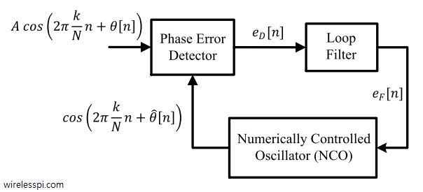
In most cases, the phase error detector is a non-linear function which makes analysis difficult. However, when the estimate is closer to the original phase, the phase error detector output can be linearized around this value and techniques from Laplace Transform can be applied to analyze and understand the loop behavior. The block diagram of a PLL operating within the linear region is redrawn below in terms of phase expressions only. Due to linearity,
\[
f(\theta) \approx k_d \theta
\]
where $k_d$ is the phase error detector gain.
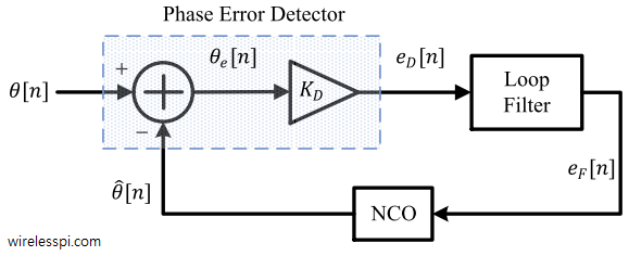
This is the steady state behavior we use for deriving our results. In Laplace domain, we can write the loop transfer function $H(s)$ as follows.
Assume that the filter transfer function is given by $G(s)$ and NCO, being an integrator, has the transform $k_0/s$. From the above figure, the NCO output $\hat \Theta(s)$ is
\[
\hat \Theta(s) = k_d G(s)\frac{k_0}{s} \left[\Theta(s) – \hat \Theta(s) \right]
\]
From here, the loop transfer function is given by
\[
H(s) = \frac{\hat \Theta(s)}{\Theta (s)} = \frac{k_d k_0 G(s)}{s+k_d k_0 G(s)}
\]
For a PI filter, we have
\[
G(s) = k_p + \frac{k_i}{s}
\]
where $k_p$ and $k_i$ are proportional and integral gains of the filter, respectively. Plugging this back in the loop transfer function, we get
\[
H(s) = \frac{k_d k_0 \left\{k_p+k_i/s\right\}}{s+k_d k_0 \left\{k_p+k_i/s\right\}} = \frac{k_dk_0k_p s + k_dk_0k_i}{s^2 + k_dk_0k_p s + k_dk_0k_i}
\]
This is the standard linear continuous-time model of a second-order PLL with closed-loop transfer function
\[
H(s) = \frac{2\zeta\omega_n s + \omega_n^2}{s^2 + 2\zeta\omega_n s + \omega_n^2}
\]
where
- $\omega_n$ is the natural frequency of the loop, and
- $\zeta$ is the damping factor.
3-dB Bandwidth
To derive the 3 dB bandwidth ($\omega_{3\text{dB}}$), we start with its closed-loop transfer function. To evaluate the frequency response, we substitute $s=j\omega$ here.
\[
H(j\omega) = \frac{j2\zeta\omega_n\omega + \omega_n^2}{-\omega^2 + j2\zeta\omega_n\omega + \omega_n^2}
\]
To make the derivation cleaner, let us normalize the frequency by defining a dimensionless frequency variable, $x = \frac{\omega}{\omega_n}$.
\[
H(jx) = \frac{1 + j2\zeta x}{(1 – x^2) + j2\zeta x}
\]
The 3 dB bandwidth is defined as the frequency where the magnitude of the transfer function drops to $1/\sqrt{2}$ of its low-frequency value (which is 1, or 0 dB). Squaring both sides means we look for the frequency where $\vert{}H(jx)\vert{}^2 = \frac{1}{2}$.
\[
\vert{}H(jx)\vert{}^2 = \frac{1 + (2\zeta x)^2}{(1 – x^2)^2 + (2\zeta x)^2} = \frac{1 + 4\zeta^2 x^2}{1 – 2x^2 + x^4 + 4\zeta^2 x^2}
\]
Next, we set the magnitude squared expression equal to $\frac{1}{2}$.
\[
\frac{1 + 4\zeta^2 x^2}{1 – 2x^2 + x^4 + 4\zeta^2 x^2} = \frac{1}{2}
\]
Cross-multiplying the above expression yields
\[
2(1 + 4\zeta^2 x^2) = 1 – 2x^2 + x^4 + 4\zeta^2 x^2
\]
which can be simplified as
\[
2 + 8\zeta^2 x^2 = 1 – 2x^2 + x^4 + 4\zeta^2 x^2
\]
Next, we rearrange all terms to one side to form a quadratic-form equation in terms of x².
\[
x^4 – (2 + 4\zeta^2)x^2 – 1 = 0, \qquad x^4 – 2(1 + 2\zeta^2)x^2 – 1 = 0
\]
Let $u = x^2$ to make the equation a standard quadratic one. Using the quadratic formula $u = \frac{-b \pm \sqrt{b^2 – 4ac}}{2a}$, we get
\[
x^2 = \frac{2(1 + 2\zeta^2) \pm \sqrt{[-2(1 + 2\zeta^2)]^2 – 4(1)(-1)}}{2}
\]
This can be written as
\[
x^2 = \frac{2(1 + 2\zeta^2) \pm \sqrt{4(1 + 2\zeta^2)^2 + 4}}{2}
\]
Factoring out the 4 from under the square root,
\[
x^2 = (1 + 2\zeta^2) \pm \sqrt{(1 + 2\zeta^2)^2 + 1}
\]
Since $x^2$ must be real and positive, we discard the negative root option. Now recall that $x = \frac{\omega}{\omega_n}$, so $x^2 = \left(\frac{\omega_{3\text{dB}}}{\omega_n}\right)^2$. Taking the square root of both sides gives
\[
\frac{\omega_{3\text{dB}}}{\omega_n} = \sqrt{(1 + 2\zeta^2) + \sqrt{(1 + 2\zeta^2)^2 + 1}}
\]
Multiplying by $\omega_n$ produces the final expression as
\omega_{3\text{dB}} = \omega_n \sqrt{1 + 2\zeta^2 + \sqrt{(1 + 2\zeta^2)^2 + 1}}
\]
For a well-damped system where $\zeta=0.707$ (a common design choice for optimal settling time and phase margin), the expression simplifies neatly to
\[
\omega_{3\text{dB}} \approx 2.06\omega_n
\]
A more useful measure of PLL bandwidth the equivalent noise bandwidth.
Equivalent Noise Bandwidth
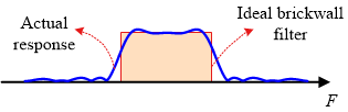
The loop frequency response strongly depends on $\zeta$ for the same $\omega_n$. Therefore, a bandwidth measure known as the equivalent noise bandwidth $B_L$ is used. Equivalent noise bandwidth is defined as the bandwidth of an ideal brickwall filter which results in the same amount of total noise power (i.e., area under the curve) as that of the actual filter. This is drawn in the figure below.
By definition, the double-sided noise bandwidth (or equivalent single-sided brick-wall bandwidth) integrates the squared magnitude of the closed-loop transfer function $H(j\omega)$.
\[
B_L = \frac{1}{2\pi} \int_{0}^{\infty} \vert{}H(j\omega)\vert{}^2 d\omega \quad \text{(in Hz)}
\]
As we saw before, the transfer function for a standard 2nd order PLL is
\[
H(s) = \frac{2\zeta\omega_n s + \omega_n^2}{s^2 + 2\zeta\omega_n s + \omega_n^2}
\]
Substituting $s=j\omega$ gives the frequency response as
\[
H(j\omega) = \frac{\omega_n^2 + j2\zeta\omega_n\omega}{(\omega_n^2 – \omega^2) + j2\zeta\omega_n\omega}
\]
To simplify the integration, define a normalized frequency variable, $x = \frac{\omega}{\omega_n}$, which implies that $d\omega = \omega_n dx$. The integration limits remain $0$ to $\infty$.
\[
H(jx) = \frac{1 + j2\zeta x}{(1 – x^2) + j2\zeta x}
\]
Next, we calculate the magnitude squared value as
\[
\vert{}H(jx)\vert{}^2 = \frac{1 + 4\zeta^2 x^2}{(1 – x^2)^2 + 4\zeta^2 x^2} = \frac{1 + 4\zeta^2 x^2}{x^4 + 2(2\zeta^2 – 1)x^2 + 1}
\]
Substitute these expressions back into the $B_L$ definition.
\[
B_L = \frac{\omega_n}{2\pi} \int_{0}^{\infty} \frac{1 + 4\zeta^2 x^2}{x^4 + 2(2\zeta^2 – 1)x^2 + 1} dx
\]
Integrals of this rational form can be solved using standard calculus tables or residue calculus. The general formula for this specific type of definite integral is given by
\[
\int_{0}^{\infty} \frac{1 + A x^2}{x^4 + B x^2 + 1} dx = \frac{\pi}{2} \frac{1 + A}{\sqrt{2 + B}}
\]
We can match our coefficients to the general formula as
- $A = 4\zeta^2$, and
- $B = 2(2\zeta^2 – 1) = 4\zeta^2 – 2$.
We substitute $A$ and $B$ into the solution to get
\[
\int_{0}^{\infty} \frac{1 + 4\zeta^2 x^2}{x^4 + 2(2\zeta^2 – 1)x^2 + 1} dx = \frac{\pi}{2} \frac{1 + 4\zeta^2}{\sqrt{2 + (4\zeta^2 – 2)}}
\]
Next, we can simplify the denominator as
\[
\sqrt{2 + 4\zeta^2 – 2} = \sqrt{4\zeta^2} = 2\zeta
\]
This reduces our integral to the following expression.
\[
\int_{0}^{\infty} \vert{}H(jx)\vert{}^2 dx = \frac{\pi}{2} \left( \frac{1 + 4\zeta^2}{2\zeta} \right)
\]
Now we can plug the evaluated integral back into the expression for $B_L$.
\[
B_L = \frac{\omega_n}{2\pi} \cdot \left[ \frac{\pi}{2} \left( \frac{1 + 4\zeta^2}{2\zeta} \right) \right]
\]
Further simplification produces the expression
\[
B_L = \frac{\omega_n}{4} \left( \frac{1 + 4\zeta^2}{2\zeta} \right)
\]
Finally, we can distribute the $2\zeta$ term in the denominator to get the final expression as
B_L = \frac{\omega_n}{2} \left( \zeta + \frac{1}{4\zeta} \right)
\]
For the common design baseline where $\zeta = 0.707$, the loop noise bandwidth evaluates to approximately $B_L \approx 0.53 \omega_n$.