
If beamforming has to be explained in the most succinct manner, it is the mindfulness of an antenna array where it focuses its attention towards one specific location (or a few specific locations). We find out in this article how it is achieved.
As opposed to its reputation, beamforming is not a mysterious technology. It has been used by signal processing engineers for radio applications since long. For example, Marconi used four antennas to increase the gain of signal transmissions across the Atlantic in 1901. It has also been known since 1970s that multiple antennas at the base station help simultaneous communication with several users. It was only after the advent of Multiple Input Multiple Output (MIMO) systems in mid 1990s, and then its adoption as the defining technology for 5G networks, that beamforming became a household terminology.
The confusing aspect of beamforming arises due to its inherent association with the idea of directionality that does not make sense in urban cellular networks (with buildings, trees, vehicles and other objects) posing an obstacle to the Line of Sight (LoS) paths. This is related to generalized beamforming that is described in 5G Physical Layer book. Here, we cover the concept of classical beamforming.
Background
In a cellular network like 5G, the electromagnetic energy emanating from the Tx antennas or arriving at the Rx antennas consists of the desired signal and interference signals from the perspective of a certain user. If only a Line of Sight (LoS) exists between the base station and that user, the angles in a geometrical space can act as suitable differentiators for each user.
-
- For instance, on the left of the figure below is a radiation pattern of a single isotropic antenna which radiates or receives an equal amount of power from all directions, very similar to a light bulb. In a cellular network, a device (whether base station or mobile) not intended to receive that signal still had to deal with interference coming from the transmissions directed at another device. We conclude that lots of energy is wasted in unwanted directions that could instead be utilized to boost the power to the desired user. This is where the power of focus comes in.

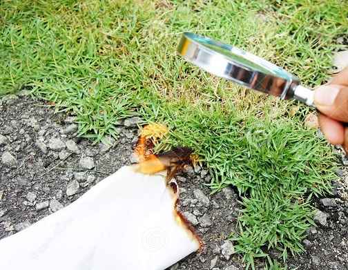
- Now shown on the right side of the figure above is an antenna array that ‘looks’ only into a particular intended direction thus minimizing the interference for other users in the same area. This is the essence of classical beamforming which is implemented through varying the phase and/or amplitude of the signal at each antenna. This is similar to the children’s experience of burning a paper with a magnifying glass under the sun as illustrated in the figure below. This demonstrates the power of focus that spreads thinner with increasing number of targets. Space based solar power might one day beam the energy harvested in space back to earth based on a similar principle (as Isaac Asimov suggested in his story The Last Question: All Earth ran by invisible beams of sunpower coming from a small station, one mile in diameter, circling the Earth at half the distance of the Moon).

A Simple Summation of Signals
This brings us to the question about the origin of beams.
- How do multiple antennas ‘look’ into particular directions?
- Why the final radiation pattern comes from the Fourier Transform?
- Why do the overall radiation characteristics depend on both the individual elements as well as the size and configuration of the antenna array?
This is what we explain next based on the following assumptions: linear array, far field transmission, and isotropic radiation patterns.
At the Tx side, this implies that the antenna array is excited by a current source according to the modulated information riding on a carrier frequency and then each element radiates equal energy in all directions. Such isotropic radiation patterns are illustrated in the figure below for a 4-element array. It is evident that the maximum gain occurs in the direction where their patterns overlap with each other. This angle is $0^\circ$ in the scenario shown here. Also notice from the figure that a mirror beam, known as a backlobe, should be created in the opposite direction (i.e., $180^\circ$) due to the isotropic antennas assumption. In practice, this backlobe is suppressed by the use of more directional antenna elements. Coming back to our setup, the unique range for the array pattern is from $-90^\circ$ to $+90^\circ$. The reason why such a superposition results in shaped beams will be discussed shortly.

At the Rx side, the array of isotropic antennas is equally receptive to planar waves arriving from all directions which excites each element in proportion to the variations in the incoming electromagnetic wave. A signal level interpretation of the beamforming process is illustrated in the figure below from a Rx viewpoint. The signal processing operations are drawn from right to left to stay consistent with $0^\circ$ on the right side as the angle of arrival. Here, a sinusoidal wavefront representing the amplitude variations arrives at our antenna array from an angle of $0^\circ$. This means that the signals generated in each element are in phase with each other. This phase relation is shown with the help of a dashed red line in the figure crossing the respective waveforms. Therefore, when the outputs from each antenna are added together, there is a coherent summation that increases the output amplitude. In our simplistic scenario, they are all the same signal $r_0$!
\[
z = \sum _{n=0}^{3} r_n = \sum _{n=0}^{3} r_0 = 4r_0
\]
Clearly, this cumulative signal carries an amplitude in proportion to the size of the antenna array, a factor of $4$ in this figure. This is represented by a larger beam at $0^\circ$ and smaller beams on the sides in the above figure. We will now formally compute the array gain thus achieved.

One problem in the previous setup is that coherent summation with aligned phases happens only if the signal arrives at an angle of $0^\circ$. From the Tx perspective, how should we focus the signal energy towards a Rx at another angle? To answer these questions, we first find out what happens when the signal arrives from a different angle.
Phase Misalignment
Imagine a planar wavefront arriving from a sufficiently distant Tx towards the Rx array at one particular angle. In such a scenario, there will be a relative delay in the wavefront reaching each antenna element and therefore coherent summation is not possible. As an example, figure below draws a plane wave arriving at an angle of $26^\circ$ with the antenna array. If $\tau_0=0$ is the time at which the wavefront reaches the topmost reference element 0, the time delays it takes to reach the antenna elements 1, 2 and 3 are given by $\tau_1$, $\tau_2$ and $\tau_3$, respectively. This causes a misalignment of the signal copies out of each array element and at the input of the summation block. This phase misalignment is indicated by a slanted dashed line going through the waveforms in the figure below. As a consequence, all the waveforms add without phase alignment and there is no array gain achieved at the final output, illustrated through a low amplitude signal as the output waveform.

Nonetheless, this does not mean that an antenna array can ‘look’ for the target signal into one fixed direction only, as we find out next.
Introducing Time Delays
In this regard, simple signal processing techniques can be applied to steer the beam in any direction with maximum gain while placing nulls in the directions of interference. This is one of main benefits of an antenna array (i.e., a spatially sampled signal analogous to time domain sampling) over a single large antenna (i.e., a continuous spatial signal analogous to a continuous-time signal).
To see how beam formation works, refer to the figure below and suppose that the antenna array is in transmission mode.

- The last array element, 3 in this figure, sends the signal first.
- The second last element 2 starts transmitting with a delay of $\tau_1$ seconds.
- The elements 1 and 0 subsequently delay their transmissions by $\tau_2$ and $\tau_3$ seconds, respectively.
How are these delays computed such that the antenna array looks at a target direction will be discussed shortly. Here, notice that although these waves are still traveling in all directions due to the isotropic nature of the individual elements, the overlapping points representing the same phase of the waves are now tilted towards a direction of $26^\circ$. We say that the combined wavefront travels at an angle of $26^\circ$ and the antenna array is now ‘looking’ into that particular direction.
You can see this beam formation process yourself by conducting a little experiment at home. Take a bucket of water (or a pool of water somewhere after rainfall) and throw two stones in it in succession at slightly different places. Holding the two stones together in one hand and releasing them at the same time from a vertically tilted position is also possible for a shorter delay. The water waves will spread out in all directions but the crest and trough formation will show a direction in proportion to the delay between the two stones.

It is clear from the above figures that the element delays are integer multiples of a single delay $\tau$ between any two adjacent antennas (this is only true for a uniform array).
To understand the signal level interpretation of this phenomenon, consider the array in the figure below from a Rx viewpoint now where the signal is arriving from the same angle.

Reference Time: Assign time $\tau_0=0$ to the instant the wavefront reaches the reference element 0.
Arriving Delays: Let times $\tau_1$, $\tau_2$, and $\tau_3$ denote the instants the wavefront reaches the array elements 1, 2 and 3, respectively. This means that with respect to element 0, the signal is delayed by $\tau_1$ at antenna 1, $\tau_2$ at antenna 2 and $\tau_3$ at antenna 3 (as a word of caution, these times of arrival are not the ones shown in delay blocks after the array output in the above figure.
Steering Delays: Remember that we can delay a signal in time but cannot advance it in a strictly real-time application. The strategy hence is to introduce the steering delays in reverse order of arriving delays.
- Taking the last element 3 as a reference for steering delays, we can assign a steering delay of $\tau_0=0$ to antenna 3 in the above figure.
- Similarly, a delay of $\tau_1$ is inserted at antenna 2 which aligns its waveform in phase with that at antenna 3.
- Finally, the signals at antennas 1 and 0 can be delayed by $\tau_2$ and $\tau_3$ seconds, respectively.
Observe the output signal of delay blocks in the above figure where they are all aligned to waveform at antenna 3 (shown by the vertical dashed line), not with the waveform at antenna 0.
Coherent Summation: Now the waveforms out of all the time delay blocks are phase aligned with each other. A summation block produces a coherent summation with an amplitude gain according to the number of antennas. This is shown as the waveform at the right of the above figure.
Next, to apply the steering delays described above, we need to compute the expressions for the time delays $\tau_1$, $\tau_2$, $\cdots$, required at each antenna element. This is what we do now.
Computing the Time Delays
To initially keep the description simple, a $d$-spaced vertical array with two antenna elements is drawn in the figure below. A planar wave (implying that the source is situated at a large distance from this array) arrives at an angle $\theta$ with the upper antenna chosen as the reference point. It is clear that the wave has to travel an extra distance to reach the lower antenna as compared to the reference point. How is this distance computed?

For this purpose, first notice that the angle between the vertical array axis and the arriving wavefront is the same as the angle of arrival $\theta$ between the horizontal axis and the direction of travel of that wave. This is because an angle between two lines is equal to the angle between their respective perpendiculars. From simple trigonometry, the extra distance traveled by the wave in the above figure to reach the lower antenna element is given by
\[
\text{Extra distance} = d \sin \theta
\]
Keep in mind that when the wavefront makes an angle $\theta$ with respect to the perpendicular to the array axis, the incremental distance term is expressed by $\sin \theta$ as above. You will see an alternative term $\cos \theta$ in many resources that arises from $\theta$ being defined as an angle with respect to the array axis itself.
If $c$ is the speed of an electromagnetic wave in the air, then the extra time to travel is the ratio of the extra distance to this speed and is denoted by $\tau$. With reference to antenna 1, we call it $\tau_1$ as well.
\begin{equation}\label{equation-time-array}
\tau = \tau_1 = \frac{\text{Distance}}{\text{Speed}} = \frac{d \sin \theta}{c}
\end{equation}
For larger arrays in a similar manner, the delays are integer multiples of a single value $\tau$ due to the uniformity of the array. In general,
\begin{equation}\label{equation-tau-n}
\tau_n = n \tau = n\frac{d \sin \theta}{c}
\end{equation}
Antenna Phase Shifts
If the signal arriving at the reference point (antenna element 0) is denoted as $r_0(t)$, how exactly is it related to the signal expression arriving at antenna element 1 and given by $r_1(t)$? Taking into account the extra travel time of $\tau$ as compared to the reference, we can write this expression from Eq (\ref{equation-time-array}).
\begin{equation}\label{equation-s0-s1-delay}
r_1(t) = r_0(t-\tau) = r_0\left(t-\frac{d\cdot \sin \theta}{c}\right)
\end{equation}
Let us take $r_0(t)$ as the most general narrowband signal, i.e., a complex sinusoid with frequency $F$. We now use the lesson learned through complex signals why the delays (an undesirable option) can be converted into multiplications (well suited to our digital processing architectures).
For a narrowband transmission, the signal $r_0(t)$ as a complex sinusoid can be written as
\[
r_0(t) = e^{j\omega t}
\]
Now the signal $r_1(t)$ with a delay of $\tau$ seconds is given by
\begin{equation}\label{equation-complex-product}
r_1(t) = e^{j\omega (t-\tau)} = \underbrace{e^{j\omega t}}_{r_0(t)}\cdot \underbrace{e^{-j\omega\tau}}_{a_1}
\end{equation}
which is simply a product between the original signal $r_0(t)$ and a complex constant $e^{-j\omega \tau}$! Clearly, a phase shift of $\omega \tau$ occurs at the first antenna element. Let us define this antenna phase shift as $u=\omega \tau$. From Eq (\ref{equation-time-array}), recall that $\tau=d\sin\theta/c$. Moreover, the wavelength $\lambda$ of the complex sinusoid is related to the frequency $F$ and the speed of an electromagnetic wave $c$ by $\lambda\cdot F_C=c$. As a consequence, $\omega=2\pi F=2\pi c/\lambda$ and
\[
u = \omega\tau = 2\pi F ~ \frac{d\sin\theta}{c} = 2\pi \frac{d\sin\theta}{\lambda}
\]
The variable $u$ then becomes
u = 2\pi \frac{d\sin\theta}{\lambda}
\end{equation}
I could have denoted this antenna phase shift $u$ with something like $\phi$ but that could potentially cause confusion in reader’s mind with the actual beam direction $\theta$. In conclusion, a complex sinusoid $r_0(t)$ appearing at the reference antenna $0$ also appears at the reference antenna $1$ but with a slight difference. It is
- delayed by $\tau$, or equivalently,
- phase shifted by $u=\omega \tau$, or equivalently,
- multiplied with a complex number $a_1$ given by Eq (\ref{equation-complex-product}).
Generalizing this observation, the complex sinusoid $r_0(t)$ also appears at antennas $2$, $3$, $\cdots$ $N_R-1$ but it is multiplied with a complex scalar $a_n$ that can be given by using $\tau_n=n\tau$ and hence $\omega \tau_n=\omega \tau n=un$. These complex scalars — combined in a vector form — are known as an array response vector which can be written in complex notation as
\begin{equation}\label{equation-complex-array-response}
a_n = e^{-j2\pi \frac{d\sin \theta}{\lambda}n} = e^{-jun}
\end{equation}
In summary, these delays can be seen as an array response vector for narrowband signals that induce a multiplication of element output $r_n(t)$ with a complex scalar $a_n$ of Eq (\ref{equation-complex-array-response}). Physical beamforming deals with compensating for these complex products.
Aligning the Phases
Since our purpose is to remove this phase shift arising from the arriving time delays, the weights $w_n$ are chosen as conjugates of $a_n$ in this scheme, $w_n=a_n^*$. Also, a multiplication of two complex numbers implies a product of their magnitudes while addition of their phases. Applying this rule to multiply $a_n$ with $w_n$, we get
\[
\begin{aligned}
|w_n\cdot a_n| &= |a_n^*\cdot a_n| = |a_n|^2 = 1 \\
\measuredangle \left(w_n\cdot a_n\right) &= \measuredangle w_n + \measuredangle a_n = +un-un = 0
\end{aligned}
\]
for each array element $n$. The effect of delays has vanished! The product $w_n\cdot a_n$ simply becomes a real number $1$ with zero phase that can be compactly written as
\begin{equation}\label{equation-wi-ai}
w_n\cdot a_n = 1
\end{equation}
A major consequence of the above result is that the output from each antenna has the delay arising from the extra distance $d\sin \theta$ removed and all the waveforms can be added in phase. Importantly, this is accomplished through much simpler complex multiplications performing the same function as time delays for narrowband signals. A block diagram for this approach is illustrated in the figure below along with the waveforms involved at various stages.

Here is a simple mathematical derivation for the gain.
- From Eq (\ref{equation-s0-s1-delay}), we know that the signal at each antenna $r_n(t)$ is a delayed version of the narrowband signal $r_0(t)$ arriving at the reference antenna.
\[
r_n(t) = r_0(t-\tau_n)
\] - Also, Eq (\ref{equation-complex-product}) can be generalized to represent that delay as a complex product.
\[
r_n(t) = a_n\cdot r_0(t)
\] - The beamformer multiplies the antenna signals $r_n(t)$ with complex weights $w_n$ followed by a summation.
\[
z = \sum _{n=0}^{3}w_n\cdot r_n(t)
\] - Therefore, the resultant signal at the beamformer output is given by
\[
\begin{aligned}
z &= \sum _{n=0}^{3}w_n\cdot r_0(t-\tau_n) = \sum _{n=0}^{3}w_n\cdot a_n \cdot r_0(t) \\
&= \sum _{n=0}^{3}r_0(t) \hspace{1in} \text{as }w_n\cdot a_n=1 \text{ from Eq (\ref{equation-wi-ai})}\\
&= 4\cdot r_0(t)
\end{aligned}
\]
thus yielding a gain of $4$ here.
Now we can see the crux of classical beamforming in the simplest setting: It is phase shifting the output of each element prior to summation. Since it forms directional beams in actual space, physical beamforming is a good term to describe the concept and can be called the mindfulness of the array. For narrowband signals, this phase shifting is an approximation but it is widely used and gives very good results in most situations.
For broadband signals on the other hand, the phase shifts alone are insufficient and filters are required in each path that perform the equivalent of time-delay beamforming task. In addition, there are three dominant architectures to implement the system, namely analog, digital and hybrid approaches.


This is a wonderful presentation on antenna array processing. I am simulating a similar system where i consider two transmitters one at 30 degree transmitting BPSK modulated OFDM signal (NFFT = 4096, CP = 288, Nsym =14). Similarly another transmitter transmitting QPSK modulated OFDM signal with same config parameters. At the transmitter, after IFFT, I am upconverting the signal to 1 Ghz and at the receiver, I am providing the delay based on the AoA and the receive antenna element. After providing the delay, I am combining both the signals, perform FFT. After FFT, I am doing a steering vector based combining to detect the BPSK and QPSK signal separately. But the BER is affected very badly compared to the scenario where there is only one transmitter.
Can you suggest me any proper algorithm to separate out the QPSK and BPSK signals after FFT at the receiver?
You need to separate them using spatial domain signal processing, not time domain signal processing. Otherwise, the transmissions interfere with each other where you are combining them.