Recall that classical or physical beamforming is based on calculating the differences in wave arrival times of a signal between antenna array elements and compensating for these delays through signal processing techniques that steer the beams in any desired direction. There are two main candidates for this purpose: Phase shifting and True Time Delays (TTD).
We saw in that article on beamforming that phase shifts implemented through a set of complex multipliers are incapable of beamforming over the entire bandwidth of a signal. Why? The intuitive reason is clear from a signal level view. In the narrowband scenario, the same signal reached the array with no change except a progressive delay from one antenna to the next. As we see in the figure below, the baseband signal arriving at the reference antenna $0$ has changed during the time interval $\tau$ it takes to reach antenna $1$. As a consequence, individual array elements here observe different versions of the complex baseband signal, resulting in a phenomenon known as beam squint.

On the other hand, introducing time delays in signal paths is a general solution that is explored further here. There are two main technologies available for this purpose: analog and digital. An analog solution to introduce the above mentioned time delays is to insert a set of switched transmission lines with incremental lengths behind each antenna element or a group of elements. However, there are two main problems with this approach.
- A large number of such delay lines requires a complex switching network and the resultant switched lines make the equipment bulky and expensive, particularly for 5G systems incorporating massive MIMO at the base stations.
- No component is perfect and the differences in dispersion in various transmission line sections lead to inaccurate beamforming.
Coming to the digital side, there are two main techniques to form beams for broadband signals.
Spatial Filtering
In addition to the narrowband beamforming that caters for the center frequency through spatial sampling, an architecture shown in the figure above samples the signal in both space and time. This enables two-dimensional filtering and combines regular narrowband beamforming with time domain filtering, similar to how a Finite Impulse Response (FIR) filter is implemented in DSP applications. Observe that each antenna element is attached to its own filter due to which the weights $w_{n,l}$ are denoted by two indices, the first across space and the other across time. The cumulative signal out of all the branches is given by
\[
z(p) = \sum _{n=0}^{3}~\sum_{l=0}^2 w_{nl}\cdot r_n(p-l)
\]
where the index $l$ indicates time indices and $p$ denotes the current time. This is also known as a tapped delay line structure. Each such branch by necessity needs to have separate RF electronics and ADC forming an efficient yet expensive fully digital solution.
For example, a bank of time domain FIR filters can be used that progressively delays the incoming waveforms at their respective antennas. One such example is shown in the figure below. From the impulse responses, it is clear that the zeroth filter produces a sample that is exactly at the peak (i.e., there is no delay introduced). For each successive array element, there is a shift in the peak towards the left, as shown by dashed green lines in this figure. This is why these filters are said to provide linear phase shifts producing the time delays that perform a beamforming task similar to multi-rate filters. The drawback is that processing the signal out of each antenna through a digital filter is quite complex.

Next, I describe a beautiful downsampling analogy to this beamforming process.
This methodology is the space counterpart to downsampling a digital signal in time domain (feel free to skip this note if you do not have a background in DSP). Readers with a DSP knowledge will enjoy comparing the successive delays in the previous beamforming figures with a downsampling architecture shown in the figure below which is taken from my wireless communications book. The signal delivered to the bottom path is the current input sample. The signal delivered to the filter one path up is the next input sample. With each clock cycle, the commutator moves upwards traversing the successive paths of the polyphase partition and delivering next arriving samples with one sample delay. The final summation at the end produces the desired signal at a reduced rate. This can be considered as beamforming in delay domain.

A reader with DSP background will recognize the similarity to sample rate conversion in time domain as described by Fred Harris.
”This phase sensitive summation aligns contributions from the desired alias to realize the processing gain of the coherent sum while the remaining alias terms, which exhibit rotation rates corresponding to $M$ roots of unity, are destructively canceled in the summation.”
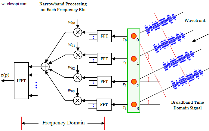
Frequency Domain Beamforming
The spatial filtering structure is more complex than simple narrowband beamforming which generates an interest in an architecture that handles broadband signals in a manner similar to a narrowband structure. This is accomplished through frequency domain beamforming in the figure below. in which a Discrete Fourier Transform (an efficient implementation of which is the Fast Fourier Transform, or FFT) is taken at the output of each element. This data is processed through its own beamformer before returning to time domain through an iFFT. While both time domain and frequency domain beamformers achieve the same purpose, frequency domain solution is more efficient beyond a certain filter order. Moreover, it has been shown to be less sensitive to coefficient quantization and more suited to VLSI implementation. Frequency domain beamforming is important for 5G systems in the context of mmWave OFDM systems with massive bandwidths. Frequency domain is also suited to the most flexible digital solution as compared to analog and hybrid architectures.

We saw before how in an OFDM system, the modulation symbols are considered to be in frequency domain and an inverse Fast Fourier Transform (iFFT) generates the actual time domain waveform. Therefore, there are two possible options to execute digital beamforming: frequency domain and time domain. This is illustrated in the figure below where the beamforming operations before the iFFT fall in the frequency domain while the operations after the iFFT belong to time domain beamforming.

The importance of frequency domain beamforming comes from the implementation of the process in a frequency selective manner, i.e., different precoding weights can be associated with separate subcarriers, thus providing maximum flexibility in both time and frequency domains. Finally, the whole beamforming operation can also be broken down into different subsets which can then be individually executed at different stages. The actual implementation can be done through an analog, digital or a hybrid approach. While the current trend in 5G systems at mmWave bands is a hybrid architecture, a fully digital architecture will dominate all the bands in the near future.