
Correlation is a foundation over which the whole structure of digital communications is built. In fact, correlation is the heart of a digital communication system, not only for data detection but for parameter estimation of various kinds as well. Throughout, we will find recurring reminders of this fact.
As a start, consider from the article on Discrete Fourier Transform that each DFT output $S[k]$ is just a sum of term-by-term products between an input signal and a cosine/sine wave, which is actually a computation of correlation. Later, we will learn that to detect the transmitted bits at the receiver, correlation is utilized to select the most likely candidate. Moreover, estimates of timing, frequency and phase of a received signal are extracted through judicious application of correlation for synchronization, as well as channel estimates for equalization. Don’t worry if you did not understand the last sentence, as we will have plenty of opportunity on this website to learn about these topics.
By definition, correlation is a measure of similarity between two signals. In our everyday life, we recognize something by running in our heads its correlation with what we know. Correlation plays such a vital and deep role in diverse areas of our life, be it science, sports, economics, business, marketing, criminology or psychology, that a complete book can be devoted to this topic.
"The world is full of obvious things which nobody by any chance ever observes."
For all of Sherlock Holmes’ inferences, his next step after observation was always correlation. For example, he accurately described Dr James Mortimer’s dog through correlating some observations with templates in his mind:
"$\cdots$ and the marks of his teeth are very plainly visible. The dog’s jaw, as shown in the space between these marks, is too broad in my opinion for a terrier and not broad enough for a mastiff. It may have been — yes, by Jove, it is a curly-haired spaniel."
As in the case of convolution, we start with real signals and the case of complex signals will be discussed later.
Correlation of Real Signals
The objective of correlation between two signals is to measure the degree to which those two signals are similar to each other. Mathematically, correlation between two signals $s[n]$ and $h[n]$ is defined as
corr[n] = \sum \limits _{m = -\infty} ^{+\infty} s[m] h[m-n]
\end{equation}
where the above sum is computed for each $n$ from $-\infty$ to $+\infty$. The process of correlation can be understood with the following steps.
- Selecting the time shift: First, notice from its definition above that there are two indices, $n$ and $m$. The index $m$ is the summation index and the index $n$ is the variable used for the signal shift.
\begin{equation*}
h[m-n]
\end{equation*} - Sample-by-sample product: Keep $s[m]$ where it is and compute the product
\begin{equation*}
s[m]\cdot h[m-n]
\end{equation*}
The only nonzero values will be at the indices $m$ where the two signals overlap. - Sum: Add all these sample-by-sample products to generate the correlation output at the shift $n$.
\begin{equation*}
corr[n] = \sum \limits _{m = -\infty} ^{+\infty} s[m] h[m-n]
\end{equation*} - Repeat: Repeat the above process for all possible time shifts $n$.
Intuitively, this summation of sample-by-sample products computes the level of similarity between the two signals at each time shift. For example, if $s[n]$ is correlated with $s[n]$, the two signals are exactly the same for time shift $0$ and the correlation output will be the sum of squared samples, i.e., energy in the signal $s[n]$.
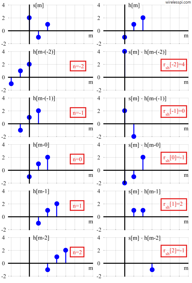
An example of correlation between two signals
\begin{align*}
s[n] &= [2~~ -1~~1] \\
h[n] &= [-1~~ 1~~ 2]
\end{align*}
is shown in Figure below. In the left column, the signal $s[m]$ is copied with shifted versions of $h[m]$ to demonstrate the overlap between the two, while the shift $n$ is shown in the text box for each $n$. If you follow the steps described above, you will find the results $corr[n]$ in the text boxes on the right column of the figure.
\begin{equation*}
r[n] = [4 ~~ 0 ~~~-1 ~~~2~~-1]
\end{equation*}
Since we said that the correlation is the heart of a digital communication system, we denote correlation operation by $\heartsuit$ as
\begin{equation}\label{eqIntroductionCorrelation2}
corr[n] = s[n] ~\heartsuit~ h[n]
\end{equation}
Note that
\begin{equation}\label{eqIntroductionCorrelationCommutative}
s[n] ~\heartsuit~ h[n] \neq h[n] ~\heartsuit~ s[n]
\end{equation}
This can be verified by plugging $p = m-n$ in Eq \eqref{eqIntroductionCorrelation1} which yields $m = n+p$ and hence
\begin{align*}
\sum \limits _{p = -\infty} ^{\infty} s[n+p] h[p] &= \sum \limits _{p = -\infty} ^{\infty} h[p] s[p+n] \\
& \neq \sum \limits _{m = -\infty} ^{\infty} h[m] s[m-n]
\end{align*}
Nevertheless, it can be deduced that Eq \eqref{eqIntroductionCorrelation1} is equivalent to
\begin{equation}\label{eqIntroductionCorrelation3}
corr[n] = \sum \limits _{m = -\infty} ^{\infty} s[m+n] h[m]
\end{equation}
Correlation of Complex Signals
Correlation between two complex signals $s[n]$ and $h[n]$ can be understood through writing Eq \eqref{eqIntroductionCorrelation1} in $IQ$ form. However, another difference from convolution is that one signal is conjugated as
\begin{align}
corr[n] &= s[n] ~\heartsuit~ h[n] \nonumber \\
&= \sum \limits _{m = -\infty} ^{\infty} s[m] h^*[m-n] \label{eqIntroductionComplexCorrelation1}
\end{align}
where conjugate of a signal negates the $Q$ arm of $h[m-n]$. We shortly see the need to introduce the conjugate operation in the second signal. The above equation can be decomposed through utilizing the multiplication rule of complex numbers.
\begin{align} \label{eqIntroductionComplexCorrelation2}
corr_I[n]\: &= s_I[n] ~\heartsuit~ h_I[n] + s_Q[n] ~\heartsuit~ h_Q[n] \\
corr_Q[n] &= s_Q[n] ~\heartsuit~ h_I[n] – s_I[n] ~\heartsuit~ h_Q[n]
\end{align}
The actual computations can be written as
\begin{align} \label{eqIntroductionComplexCorrelation3}
corr_I[n]\: &= \sum \limits _{m = -\infty} ^{\infty} s_I[m] h_I[m-n] + \sum \limits _{m = -\infty} ^{\infty} s_Q[m] h_Q[m-n] \\
corr_Q[n] &= \sum \limits _{m = -\infty} ^{\infty} s_Q[m] h_I[m-n] – \sum \limits _{m = -\infty} ^{\infty} s_I[m] h_Q[m-n]
\end{align}
Due to the identity $\cos A \cos B + \sin A \sin B = \cos (A-B)$, a positive sign in $I$ term indicates that phases of the two aligned-axes terms are actually getting subtracted. Obviously, the identity applies in above equations only if magnitude can be extracted as common term, but the concept of phase-alignment still holds. Similarly, the identity $\sin A \cos B – \cos A \sin B = \sin (A-B)$ implies that phases of the two cross-axes terms are also getting subtracted in $Q$ expression. Hence, a complex correlation can be described as a process that
- computes $4$ real correlations: $I ~\text{corr}~ I$, $Q ~\text{corr}~ Q$, $Q ~\text{corr}~ I$ and $I ~\text{corr}~ Q$
- subtracts by phase anti-aligning the $2$ aligned-axes correlations ($I$ $\diamond$ $I$ + $Q \diamond Q$) to obtain the $I$ component
- subtracts the $2$ cross-axes correlations ($Q ~\text{corr}~ I$ – $I ~\text{corr}~ Q$) to obtain the $Q$ component.
Now it can be inferred why a conjugate was required in the definition of complex correlation but not complex convolution. The purpose of correlation is to extract the degree of similarity between two signals, and whenever $A$ is close to $B$,
\begin{align*}
\cos(A-B) &\approx 1 \\
\sin(A-B) &\approx 0
\end{align*}
thus maximizing the correlation output.
Correlation and Frequency Domain
Just like convolution, there is an interesting interpretation of correlation in frequency domain. As before, DFT works with circular shifts only due to the way both time and frequency domain sequences are defined within a range $0 \le n, k \le N-1$.
As always, we apply Eq \eqref{eqIntroductionCorrelation1} to DFT definition. The derivation is similar to convolution.
Circular correlation between two signals in time domain is equivalent to multiplication of the first signal with conjugate of the second signal in frequency domain because
\begin{equation*}
s[n] ~\boxed{\text{corr}}~ h[n] = s[n] \circledast h^*[-n]
\end{equation*}
which leads to
\begin{equation}
s[n] ~\boxed{\text{corr}}~ h[n] ~\rightarrow ~ S[k] \cdot H^*[k] \label{eqIntroductionCorrelationMultiplication}
\end{equation}
and the relation between $h^*[-n]$ and $H^*[k]$ can be established through the DFT definition.
Cross and Auto-Correlation
The correlation discussed above between two different signals is naturally called cross-correlation. When a signal is correlated with itself, it is called auto-correlation. It is defined by setting $h[n] = s[n]$ in Eq \eqref{eqIntroductionComplexCorrelation1} as
\begin{align}
r_{ss}[n] &= s[n] ~\text{corr}~ s^*[n] \nonumber \\
&= \sum \limits _{m = -\infty} ^{\infty} s[m] s^*[m-n] \label{eqIntroductionAutoCorrelation}
\end{align}
An interesting fact to note is that
\begin{align}
r_{ss}[0] &= \sum \limits _{m = -\infty} ^{\infty} s[m] s^*[m] \nonumber \\
&= \sum \limits _{m = -\infty} ^{\infty} |s[m]|^2 \nonumber \\
&= E_s \label{eqIntroductionAutoCorrelationEnergy}
\end{align}
which is the energy of the signal $s[n]$.
Remember that another signal can have a large amount of energy such that the result of its cross-correlation with $s[n]$ can be greater than the auto-correlation of $s[n]$, which intuitively should not happen. Normalized correlation $\overline{r}_{sh}[n]$ is defined in Eq \eqref{eqIntroductionCorrelationNormalized} in a way that the maximum value of $1$ can only occur for correlation of a signal with itself.
\begin{align}
\overline{r}_{sh}[n] &= \frac{\sum \limits _{m = -\infty} ^{\infty} s[m] h^*[m-n]}{\sqrt{\sum \limits _{m = -\infty} ^{\infty} |s[m]|^2} \cdot \sqrt{\sum \limits _{m = -\infty} ^{\infty} |h[m]|^2}} \nonumber \\
&= \frac{1}{\sqrt{E_s} \cdot \sqrt{E_h}} ~~ \sum \limits _{m = -\infty} ^{\infty} s[m] h^*[m-n] \label{eqIntroductionCorrelationNormalized}
\end{align}
In this case, regardless of the energy in the other signal, its normalized cross-correlation with another signal cannot be greater than the normalized auto-correlation of a signal due to both energies appearing in the denominator.
Spectral Density
Taking the DFT of auto-correlation of a signal and utilizing Eq \eqref{eqIntroductionCorrelationMultiplication}, we get
\begin{equation}\label{eqIntroductionSpectralDensity}
r_{ss}[n] \quad \rightarrow \quad S[k] \cdot S^*[k] = |S[k]|^2
\end{equation}
The expression $|S[k]|^2$ is called Spectral Density, because from Parseval relation in the article on DFT Examples that relates the signal energy in time domain to that in frequency domain,
\begin{equation*}
E_s = \sum _{n=0} ^{N-1} |s[n]|^2 = \frac{1}{N} \sum _{n=0} ^{N-1} |S[k]|^2
\end{equation*}
Thus, energy of a signal can be obtained by summing the energy $|S[k]|^2$ in each frequency bin (up to a normalizing constant $1/N$). Accordingly, $|S[k]|^2$ can be termed as energy per spectral bin, or spectral density.
From the above discussion, there are two ways to find the spectral density of a signal:
- Take the magnitude squared of the DFT of a signal.
- Take the DFT of the signal auto-correlation.
Thank you so much, what a clear explanation!.
Glad you liked it.