In Physics, frequency in units of Hz is defined as the number of cycles per unit time. Angular frequency is the rate of change of phase of a sinusoidal waveform with units of radians/second.
\begin{equation*}
2\pi f = \frac{\Delta \theta}{\Delta t}
\end{equation*}
where $\Delta\theta$ and $\Delta t$ are the changes in phase and time, respectively. A Carrier Frequency Offset (CFO) usually arises due to two reasons. The video below also explains this concept.
- [Frequency mismatch between the Tx and Rx oscillators] No two devices are the same and there is always some difference between the manufacturer’s nominal specification and the real frequency of that device. Moreover, this actual frequency keeps changing (slightly) with temperature, pressure, age, and some other factors.
- [Doppler effect] A moving Tx, Rx or any kind of movement around the channel creates a Doppler shift that creates a carrier frequency offset as well. We will learn more about it during the discussion of a wireless channel in another post.
To see the effect of the carrier frequency offset $F_\Delta$, consider again a received passband signal consisting of two PAM waveforms in $I$ and $Q$ arms.
\begin{align}
r(t) &= v_I(t) \sqrt{2} \cos \Big[2\pi (F_C+F_\Delta) t + \theta_\Delta\Big] – v_Q(t) \sqrt{2}\sin \Big[ 2\pi (F_C+F_\Delta) t + \theta_\Delta \Big]\nonumber\\
&= v_I(t) \sqrt{2} \cos \Big[2\pi F_Ct + 2\pi F_\Delta t + \theta_\Delta\Big] – \nonumber \\ &\hspace{2in}v_Q(t) \sqrt{2}\sin \Big[ 2\pi F_C t+ 2\pi F_\Delta t + \theta_\Delta\Big]\label{eqRealWorldQAMFreqOffset}
\end{align}
Here, the impact of carrier offset can be seen as $2\pi F_\Delta t$ which is changing the phase with time. Let us look into how to find $F_{\Delta,\text{max}}$, the maximum value CFO can take.
The accuracy of local oscillators in communication receivers is defined in terms of ppm (parts per million). 1 ppm is just what it says: 1 out of $10^6$ parts. To get a feel of how big or small this number is, $10^6$ seconds translate into
\begin{equation*}
\frac{10^6~ \text{seconds}}{24~ \text{hours/day} \times 3600 ~\text{seconds/hour}} \approx 11.5~ \text{days}
\end{equation*}
Hence, $1$ ppm is equivalent to a deviation of $1$ second every $11.5$ days. This might sound entirely harmless but for the purpose of typical wireless communication systems operating at several GHz of carrier frequency $F_C$ and several MHz of symbol rates $R_M$, it is one of the major sources of signal distortion.
The ppm rating at the oscillator crystal indicates how much its frequency may deviate from the nominal value. Consider an example of a wireless system operating at $2.4$ GHz and with $\pm 20$ ppm crystals, which is a more or less standard rating. The maximum deviation of the carrier frequency at the Tx or Rx can be
\begin{equation*}
\pm \frac{20}{10^6} \times 2.4 \times 10^9 = \pm 48 \text{kHz}
\end{equation*}
However, in the worst case scenario, the Tx can be $20$ ppm above (or below) the nominal frequency, while the Rx can be $20$ ppm below (or above) the nominal frequency, resulting in the overall difference of $40$ ppm between the two. So the worst case CFO due to local oscillator mismatch in this example can be
\begin{equation*}
\pm 2 \times 48 = \pm 96 \text{kHz}
\end{equation*}
Keep in mind that this calculation is for basic precision and the actual frequency may vary depending on environmental factors, mainly the temperature and aging. Finally, a movement anywhere in the channel (whether by Tx, Rx or some other object within that environment) adds Doppler shift which can be up to several hundreds of Hz. Although this Doppler shift is much less than the oscillator generated mismatch, it severely distorts the Rx signal due to the changes it causes in the channel.
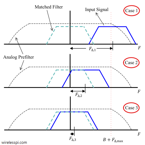
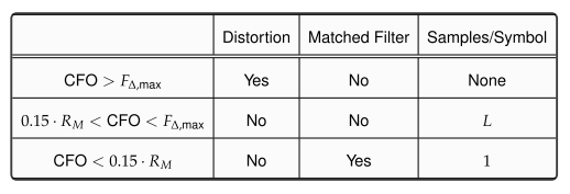
Now we turn our attention towards Figure below to differentiate between three possibilities in which $F_\Delta$ can dictate the receiver design.

Case 1: CFO $> F_{\Delta,\text{max}}$
It was illustrated in another article that an input signal at the Rx is filtered by an analog prefilter to remove the out of band noise. Ideally, the frequency response of this prefilter $G(F)$ should be flat within the frequency range
\begin{equation*}
|F| \le B + F_{\Delta,\text{max}}
\end{equation*}
so that the incoming signal can pass through in an undistorted manner (we are assuming a flat wireless channel here as well. Actual wireless channels will be discussed later). The passband width of this prefilter is designed according to the maximum CFO $F_{\Delta,\text{max}}$ expected at the Rx.
However, if the CFO is greater than $F_{\Delta,\text{max}}$, then much of the actual intended signal will be filtered out by the analog prefilter and the Rx sampled signal will not even closely resemble the Tx signal as a linear function of Tx data. No amount of signal processing can then recover the signal. Since it is an outcome of poor system design, the only remedy is to redesign the system (particularly the analog frontend) with more accurate estimates and margins for CFO and other such random distortions.
Case 2: $15\%$ of $R_M$ $<$ CFO $<$ $F_{\Delta,\text{max}}$
Since CFO $<$ $F_{\Delta,\text{max}}$, the Rx signal is within the passband of the analog prefilter $G(F)$ and suffers no distortion. However, remember from a previous post that to maximize the SNR, the Rx signal must be passed through a matched filter. This is not possible in this case because much of the Rx signal bandwidth does not sufficiently overlap with the matched filter due to the CFO being greater than $15\%$ of symbol rate $R_M$. If applied, it would remove a significant portion of the incoming signal energy.
Since Rx signal cannot be matched filtered without distorting the signal, and the signal cannot be downsampled to $1$ sample/symbol without matched filtering, it is easy to deduce that more than $1$ sample/symbol (say, $L$) is required to trace the frequency offset.
Case 3: CFO $<$ $15\%$ of $R_M$
When the signal is rotated by less than $15\%$ $R_M$, an offset cycle gets completed in less than $7$ symbols, and hence the effect of rotation on one symbol, although still significant, can now be tracked at symbol rate, or $1$ sample/symbol. In other words, matched filtering keeps most of the signal intact and as a result, symbol boundaries can be marked first (a problem known as symbol timing synchronization which we discuss in another article) before carrier frequency is estimated at the ISI-free symbol-spaced samples.
In the absence of noise, the sampled version of this mismatch in Eq \eqref{eqRealWorldQAMFreqOffset} becomes $2\pi F_\Delta nT_S$. Now Eq \eqref{eqRealWorldQAMFreqOffset} is very similar to phase rotation equation, and hence we can use directly use that result with proper substitution. The expression for the symbol-spaced samples in the presence of CFO $F_{\Delta}$ can be obtained after replacing sample time index $n$ with the symbol time index $m$.
\begin{equation*}
\begin{aligned}
z_I(mT_M) &= a_I[m] \cos 2\pi F_\Delta mT_M – a_Q[m]\sin 2\pi F_\Delta mT_M \\
z_Q(mT_M) &= a_I[m] \sin 2\pi F_\Delta mT_M + a_Q[m]\cos 2\pi F_\Delta mT_M
\end{aligned}
\end{equation*}
In the above equation,
\begin{equation*}
2\pi F_\Delta mT_M = 2\pi \frac{F_\Delta}{R_M} m = 2\pi F_0 m
\end{equation*}
where the $F_0$ is defined as the normalized Carrier Frequency Offset (nCFO): CFO normalized by the symbol rate.
\begin{equation*}
F_0 = \frac{F_\Delta}{R_M}
\end{equation*}
This normalization is very important as we saw in the last subsection. The resulting expression takes the form
\begin{equation*}
\begin{aligned}
z_I(mT_M) = a_I[m] \cos 2\pi F_0m – a_Q[m]\sin 2\pi F_0m \\
z_Q(mT_M) = a_I[m] \sin 2\pi F_0m + a_Q[m]\cos 2\pi F_0m
\end{aligned}
\end{equation*}
In polar form, this expression can be written as
\begin{equation*}
\begin{aligned}
|z(mT_M)| &= \sqrt{a_I^2[m] + a_Q^2[m]} \\
\measuredangle z(mT_M) &= \measuredangle \Big(a_Q[m],a_I[m]\Big) + 2\pi F_0 m
\end{aligned}
\end{equation*}
Notice from the above equation that a carrier frequency offset of $F_\Delta$ keeps the magnitude unchanged but continually rotates the desired outputs $a_I[m]$ and $a_Q[m]$ on the constellation plane. This is drawn for symbol-spaced samples in the scatter plot of Figures below for a $4$-QAM and $16$-QAM constellation.
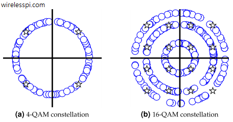
Due to this reason, a Carrier Frequency Offset (CFO), or $F_{\Delta}$, in the received signal spins the constellation in a circle (or multiple circles for higher-order modulations). This is a natural outcome since the angular frequency is defined as the rate of change of phase.
The above results are summarized in Table below.

Hello,
I am not sure if I completely understand when you say that the carrier offset can be seen as 2πF∆t in eq (1) which is changing with time. Isn’t carrier offset equal to F∆ which is a constant? E.g. in practice if the Rx frequency is 1MHz and the received signal is at 1.2MHz, the offset should be 0.2MHz.
Could you please shed some light.
Thanks
Yes, I have clarified the statement there: “the impact of carrier offset can be seen as $2\pi F_\Delta t$ which is a changing phase with time”.
Hello! Thanks for writing the article. From what I can see, the received signal has a cos component and a sin component. And the 2.pi.Fc.t term (relating to the carrier frequency) is changing with time already.
So even if we ignore the FΔ term, the vector formed by Vi and Vq is going to be rotated by 2.pi.Fc.t
And for a non-zero value of FΔ, the 2.pi.(Fc+FΔ).t term is simply going to rotate the vector (formed by Vi and Vq) faster, right?
Thanks and best regards.
You’re almost right. What you are not including here is the effect of downconversion. The Rx de-rotates the incoming signal by 2 pi Fc t so there is no such term left in the resulting signal. The only term that now rotates the signal is the frequency offset term between Tx and Rx oscillators. Hope it is clear now.
This is a bit of out of topic question. A lot of wifi sensing applications rely on a few Hz difference in frequency to detect motion. Any idea how this can be detected if the CFO in WiFi is in order of KHz?
This is an interesting question, and related to this topic too. The frequency difference for motion detection is based on Doppler Frequency, not the CFO between the Tx and Rx local oscillators. The former is typically in Hz while the latter is in kHz (as you said). If there was a single path between the Tx and the Rx, there would have been no difference between the two and they could not be separated. On the other hand, situation is different in a multipath wireless channel with Channel State Information (CSI) signatures exhibiting non-random behavior that depends on the motion of the target. Lots of different algorithms are applied to extract the motion part from Doppler shift of multipath copies in the received signal. Plz do not consider this as a sales pitch but Chapter 8 of my book on wireless communications explains this difference well with the help of nice figures.
Dear Mr. Qasim,
I am currently working on implementing OFDM using GNU Radio and USRP X300. In my experimental setup, I have one USRP serving as the transmitter (TX) and another USRP as the receiver (RX), with a separation distance of 2 meters. The transmission and reception processes are functioning correctly, and I am able to successfully retrieve the transmitted data.
However, I am encountering a challenge when it comes to analyzing the constellation phase rotation, assuming a QPSK modulation scheme, and comparing it to the constellation of the transmitted subcarriers. The issue lies in the fact that the constellation diagrams exhibit continuous rotation, forming a circular pattern. This rotation makes it difficult to determine the phase rotation accurately. It is worth noting that I am conducting the constellation analysis prior to the equalization stage, as the equalizer provides the correct QPSK constellation. I have already employed GPSDO for synchronization and have increased the SNR, yet the rotating constellation persists.
Interestingly, when I utilize the channel model block instead, I am able to observe the QPSK constellation with a phase shift caused by noise.
I kindly request your guidance and assistance in resolving this issue. Any suggestions or insights you can provide would be greatly appreciated.
Hamed, please have a look at the last figure in this article. A continuous rotation appears when the CFO is not corrected. Your system needs a CFO estimation and compensation algorithm, either feedforward or feedback.
Thanks for your reply!
I am already using the Schmidl and Cox algorithm.
That’s the problem. Schmidl and Cox can only correct a coarse CFO. You need another algorithm for fine CFO correction. Only then your constellation will stop rotating.
Okay, thanks!
Hi Qasim,
I used PLL to stop the rotation of the constellation and it worked perfectly. But I think this way removes the phase corresponding to the propagation distance. Am I right?
If yes, is there any suggestion to retrieve that information?
PLLs have been used in the estimation of propagation distance. You need to keep track of your evolved phase and use its steady-state value after convergence.
Ok, Thanks!