Demodulation – From Signals Back to Numbers

Remember that in the article on correlation, we discussed that correlation of a signal with proper normalization is maximum with itself and lesser for all other signals. Since the number of possible signals is limited in a digital communication system, we can use the correlation between incoming signal $r(nT_S)$ and possible choices $s_0(nT_S)$ and $s_1(nT_S)$ in a digital receiver. Consequently, a decision can be made in favor of the one with higher correlation. It turns out that the theory of maximum likelihood detection formalizes this conclusion that it is the optimum receiver in terms of minimizing the probability of error.

Before correlating the received signal with possible choices, it is helpful to see the correlation of a rectangular pulse shape with itself — called the auto-correlation $r_p(nT_S)$ as defined in correlation. Figure below illustrates the auto-correlation $r_p(nT_S)$ of the rectangular pulse shape whose time support is equal to a symbol duration, i.e., from $0$ to $L-1$ samples. As a consequence, its auto-correlation is a triangular pulse shape with duration clearly from $-(L-1)$ to $L-1$. From the definition of correlation,

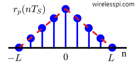
Since correlation is similar to convolution with one signal flipped, and flipping does not alter the length of a signal, the length of the correlation output is the same as convolution output, i.e., $L + L$ $-1$ $=2L-1$.

Eq \eqref{eqCommSystemPulseCorrelation} is extremely important in the design of communication systems and this term, $r_p(nT_S)$, will appear over and over again in any communications text. I will highly recommend writing it down on a piece of paper and sticking it to your laptop or book.

Now, let us compute the correlation between the received signal $r(nT_S)$ and the pulse shape $p(nT_S)$ as
\begin{align}\label{eqCommSystemSignalCorrelation}
z(nT_S) &= \sum \limits _{i=-\infty} ^{\infty} r(iT_S) p(iT_S-nT_S)
\end{align}
for all possible lags $n$. The question then is to find the optimum sampling instant: the value of $n$ that gives the best result through maximizing the correlation output. For both $r(nT_S)=s_0(nT_S)$ and $r(nT_S)=s_1(nT_S)$ with zero noise, Figure below draws the correlations for many different lags $n$.

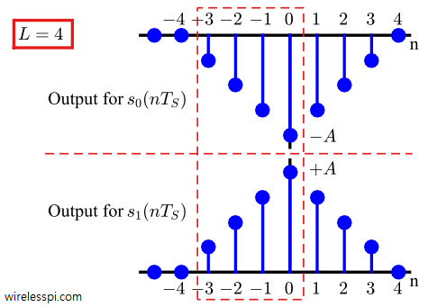
As the signal sliding occurs, the correlation outputs $z(nT_S)$ vary as
\begin{align*}
\cdots \\
n = -4 \quad &\rightarrow \quad z(-4T_S) = 0 \\
n = -3 \quad &\rightarrow \quad z(-3T_S) = \pm A/4 \\
n = -2 \quad &\rightarrow \quad z(-2T_S) = \pm 2A/4 \\
n = -1 \quad &\rightarrow \quad z(-1T_S) = \pm 3A/4
\end{align*}

\begin{align*}
n = +1 \quad &\rightarrow \quad z(+1T_S) = \pm 3A/4 \\
n = +2 \quad &\rightarrow \quad z(+2T_S) = \pm 2A/4 \\
n = +3 \quad &\rightarrow \quad z(+3T_S) = \pm A/4 \\
n = +4 \quad &\rightarrow \quad z(+4T_S) = 0 \\
\cdots
\end{align*}

It is evident that at time instant $n=0$, the output for $r(nT_S)=s_0(nT_S)$ is $-A$ and the output for $r(nT_S)=s_1(nT_S)$ is $+A$. This time instant is the point of maximum overlap where the received signal $r(nT_S)$ is completely aligned with the pulse shape. For symbol detection, only this particular sample of correlation output is needed and the rest of the samples can be discarded. This is the process of demodulation that maps a signal back to a number.

Matched Filter in Time Domain

In the above discussion, since the maximum overlap is the only sample within a symbol time $T_M$ that is required out of $L = T_M/T_S$ samples, let us substitute $n=L = T_M/T_S$ in Eq \eqref{eqCommSystemSignalCorrelation} as
\begin{align}
z(T_M) &= z(nT_S) \bigg| _{n = L = T_M/T_S} \nonumber \\
&= \sum \limits _i r(iT_S) p(iT_S-nT_S) \bigg| _{n = L = T_M/T_S} \nonumber \\
&= \sum \limits _i r(iT_S) p\Big(-(nT_S – iT_S)\Big) \bigg| _{n = L = T_M/T_S} \nonumber \\
&= r(nT_S) * p(-nT_S) \bigg| _{n = L = T_M/T_S} \label{eqCommSystemMatchedFilterOutput}
\end{align}

We conclude that the process of correlation can be implemented as convolution with a filter whose impulse response $h(nT_S)$ is a flipped version of the actual pulse shape. Most texts say that this is true only as far as the point of maximum overlap is concerned. We discuss this difference of opinion in the article on convoluted correlation between matched filter and correlator.

It is tempting to write $h(nT_S) = p(-nT_S)$, but observe from the above figure that the time base of our demodulator starts at $n=-L$ samples or $-T_M$ seconds, although a real receiver should begin processing the received signal at time $n=0$. From $n=0$, the peak or maximum overlap shifted by the same amount occurs at $n=L$ or $T_M$ seconds.

Also remember that flipping the pulse shape implies that the impulse response of this filter $p(-nT_S)$ starts at $-T_M$ seconds. Standing at $-T_M$ seconds, our filter would need future samples due to arrive at $n=0$. Since accessing future samples is not possible, the impulse response $h(nT_S)$ must be delayed by an amount $T_M$ seconds to yield $h(nT_S) = p(-nT_S+T_M)$. Remember from transforming a signal that for negative time axis as in the case here, a delay means shifting the signal to the right, which means not only that now $h(nT_S)$ starts at $n=0$ but also the filter output reaches its maximum at time $T_M$ seconds.

In summary, this flipped and delayed version of the template pulse shape is called the matched filter given by
\begin{equation*}
h(nT_S) = p(-nT_S+T_M)
\end{equation*}
Above statement is true because the pulse has real coefficients. For complex signals, complex conjugation is also required for which an intuitive explanation will be shortly described.
\begin{equation}\label{eqCommSystemMatchedFilterTime}
h(nT_S) = p^*(-nT_S+T_M)
\end{equation}

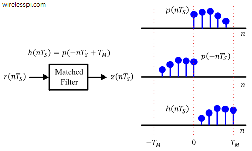
Figure above draws a matched filter for an example pulse shape. To find the matched filter output, consider that in the absence of noise, the received signal is
\begin{equation*}
r(nT_S) = \pm A \cdot p(nT_S) \\
\end{equation*}
From Eq \eqref{eqCommSystemMatchedFilterOutput},
\begin{align*}
z(T_M) &= \pm A \cdot p(nT_S) * p(-nT_S) \bigg| _{n = L = T_M/T_S} \\
&= \pm A \cdot 1 = \pm A
\end{align*}
where we utilized the fact that convolution of a signal with its flipped version is its auto-correlation which is unity at the middle point ($L^{th}$ sample). Thus, the output $z(mT_M)$ reflects the information embedded in the amplitude of the signal.

A question that immediately arises from the above derivation — but mostly not asked in communications texts — is the following: how do we know for sure that the remaining $L-1$ samples are of little use, as far as the process of demodulation is concerned? We answer this question in the next subsection during the matched filter viewpoint in frequency domain.

Expanding to a more general inference, implementing a matched filter to an incoming signal requires the following three steps:

1. Flip a true copy of the template signal.
2. Delay it by an amount that yields maximum correlation.
3. Take the complex conjugate, in case of complex signals.

Matched Filter in Frequency Domain

In frequency domain, matched filter has an interesting view as well. In some DFT properties, we learned that the DFT of a time-reversed and complex conjugated signal $s^*[(-n) \:{mod}\: N]$ is given by the complex conjugate of its DFT, i.e.,
\begin{equation}
s^*[(-n) \:{mod}\: N] ~\xrightarrow{\text{{F}}}~ S^*[k]
\end{equation}
Furthermore, as explained in the article on the concept of phase, we saw that the time shift of an input signal $s[(n-n_0) \:{mod}\: N]$ results in a corresponding phase shift $\Delta \theta (k) = -2\pi (k/N) n_0$ at each frequency of its DFT $S[k]$ with no change in magnitude.

Since $h(nT_S) = p(-(nT_S-T_M))$, and $L^{th}$ sample coincides with $T_M$, the DFT of the matched filter can be deduced by combining the above two facts as

where $N$ is the DFT size and $k$ ranges from $-N/2$ to $N/2-1$. So the DFT of the matched filter has a magnitude that is the same as the magnitude of the underlying pulse while a phase shift that is negative of the phase of the pulse DFT (which arises from taking the complex conjugate), plus an additional factor proportional to the symbol time $T_M$.

What happens when the received signal is passed through the matched filter? First, note that in presence of no noise, the received signal is expressed as
\begin{equation*}
r(nT_S) = \pm A \cdot p(nT_S) \\
\end{equation*}
whose spectrum can be written as
\begin{align*}
|R[k]| &= |A| \cdot |P[k]| \\
\measuredangle R[k] &= \measuredangle A + \measuredangle P[k]
\end{align*}
where $\measuredangle A$ is $0$ if $A$ is positive and $\pi$ if $A$ is negative. At the output of the matched filter, the convolution in time domain is multiplication in frequency domain leading to the following results.

[Magnitude] Utilizing Eq \eqref{eqCommSystemMatchedFilterFreq}, the magnitude of the matched filter output $Z[k]$ can be written as
\begin{equation*}
|Z[k]| = |R[k]|\cdot |H[k]| = |A|\cdot |P[k]| \cdot |P[k]| = |A| \cdot |P[k]|^2
\end{equation*}
Consider that for a number $b$,
\begin{align*}
b^2 > b &\quad {if}\quad b\ge 1 \\
b^2 < b &\quad {if}\quad 0\le b \le 1 \end{align*} Therefore, the matched filter has high gain at frequencies where $P[k]$ is large and low gain at frequencies where $P[k]$ is small. It can deduced that the matched filter enhances the strong spectral components and reduces the weak spectral components in $P[k]$.

[Phase] On the other hand, the phase of $Z[k]$ takes the form
\begin{align*}
\measuredangle Z[k] = \measuredangle R[k] + \measuredangle H[k] &= \measuredangle A + \measuredangle P[k] -\measuredangle P[k] – 2\pi \frac{k}{N} L \\
&= \measuredangle A – 2\pi \frac{k}{N} L
\end{align*}
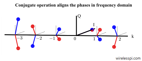
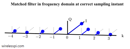
where we can notice the phase of the incoming signal being canceled by the matched filter. This phase adjustment enables all spectral components to align at sampling time instant. Figure below illustrates an example signal template and a corresponding matched filter where the blue lines represent the signal template while the red show the matched filter. Notice the same magnitude on each spectral line but exactly opposite phase. This is the reason complex conjugation is required for designing a matched filter for complex signals.

In terms of $IQ$, incorporating $\measuredangle A$ in $\pm$ form, $Z[k]$ is
\begin{align*}
Z_I[k] &= \pm A \cdot |P[k]|^2 \cos 2\pi \frac{k}{N}L \\
Z_Q[k] &= \mp A \cdot |P[k]|^2 \sin 2\pi \frac{k}{N}L
\end{align*}
where the difference of $\pm$ and $\mp$ is due to the identities $\cos (-B) = \cos B$ and $\sin (-B) = -\sin B$.

To find the output in time domain $z(nT_S)$, iDFT of $Z[k]$ needs to be taken through definition of IDFT in Discrete Fourier Transform (DFT),
\begin{equation*}
\begin{aligned}
z_I(nT_S)\: &= \frac{1}{N}\sum \limits _{k=-N/2} ^{N/2-1} Z_I[k] \cos 2\pi\frac{k}{N}n – Z_Q[k] \sin 2\pi\frac{k}{N}n \\
z_Q(nT_S) &= \frac{1}{N} \sum \limits _{k=-N/2} ^{N/2-1} Z_Q[k] \cos 2\pi\frac{ k}{N}n + Z_I[k] \sin 2\pi\frac{k}{N}n
\end{aligned}
\end{equation*}
Plugging $Z_I[k]$ and $Z_Q[k]$ in iDFT above and using identities $\cos A \cos B + \sin A \sin B = \cos (A-B)$ and $\sin A$ $\cos B$ $-$ $\cos A \sin B = \sin (A-B)$, we get
$$ \begin{equation}
\begin{aligned}
z_I(nT_S)\: &= \frac{1}{N}\sum \limits _{k=-N/2} ^{N/2-1} \pm A \cdot |P[k]|^2 \cos \left[ 2\pi \frac{k}{N} \left(n-L\right)\right] \\
z_Q(nT_S) &= \frac{1}{N} \sum \limits _{k=-N/2} ^{N/2-1} \pm A \cdot |P[k]|^2 \sin \left[ 2\pi \frac{k}{N} \left(n-L\right)\right]
\end{aligned}
\end{equation}\label{eqCommSystemMatchedFilterIDFT}$$
Sampling this matched filter output at the instant $n=L=T_M/T_S$ yields
\begin{equation*}
\begin{aligned}
z_I(T_M)\: &= \frac{1}{N}\sum \limits _{k=-N/2} ^{N/2-1} \pm A \cdot |P[k]|^2 \\
z_Q(T_M) &= 0
\end{aligned}
\end{equation*}
Figure below verifies the above finding for an all 1s sequence (no $-A$ in the received sequence). Notice that there is no $Q$ component and all frequency domain samples are perfectly aligned to contribute towards $I$ term.

Using Parseval’s relation in DFT examples that relates the signal energy in time domain to that in frequency domain,
\begin{equation*}
E_s = \sum _{n=0} ^{N-1} |s[n]|^2 = \frac{1}{N} \sum _{n=0} ^{N-1} |S[k]|^2
\end{equation*}
the matched filter output in time domain can be written as
\begin{equation*}
\begin{aligned}
z_I(T_M)\: &= \pm A \sum \limits _{n=0} ^{N-1} |p[n]|^2 = \pm A \cdot E_p\\
z_Q(T_M) &= 0
\end{aligned}
\end{equation*}
Owing to the unit energy pulse $E_p=1$,
\begin{equation*}
\begin{aligned}
z_I(T_M)\: &= \pm A \\
z_Q(T_M) &= 0
\end{aligned}
\end{equation*}
and hence the modulated information is retrieved through the amplitude of the matched filter output.

Optimality of Peak Sample

From this derivation in frequency domain, although we obtained the same result as in time domain, we get an additional insight into the operation of a digital receiver. That insight arises from answering the question asked in time domain viewpoint of the matched filter: as far as the process of demodulation is concerned, why do we discard the remaining $L-1$ samples? Why can’t we process them in a manner that improves the symbol estimate?

For the case where an all 1s sequence is transmitted (no $-A$ in the received sequence) and signal in Eq \eqref{eqCommSystemMatchedFilterIDFT} is sampled at a different time instant instead of $n=L$, say at $n=L-1$, we can trace the following sequence of steps.

• From Eq \eqref{eqCommSystemMatchedFilterIDFT},
  \begin{equation*}
  \begin{aligned}
  z_I(nT_S)\: &= \frac{1}{N}\sum \limits _{k=-N/2} ^{N/2-1} \cdot |P[k]|^2 \cos 2\pi \frac{k}{N} \\
  z_Q(nT_S) &= \frac{1}{N} \sum \limits _{k=-N/2} ^{N/2-1} \cdot |P[k]|^2 \sin 2\pi \frac{k}{N}
  \end{aligned}
  \end{equation*}
  which is nothing but a linear phase shift arising in all frequency bins due to sampling the output one unit of time earlier.

  Now, the $Q$ component of the output $z_Q(nT_S)$ is not zero. We can say that a part of the actual signal energy — that should have appeared in $I$ branch — has leaked into the $Q$ arm. The $I$ arm with reduced energy is not optimal anymore for symbol detection. This is drawn in Figure below. Notice that the spectral components have been rotated by symmetrical phase $2\pi k/N$ due to a time difference of $1$ sample.

  

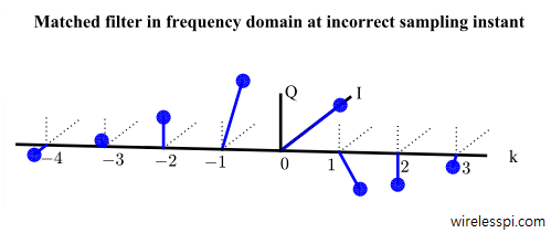
  This non-zero $Q$ sample also reveals an interesting point. In time domain, all the samples of the correlation result are less in magnitude than the peak due to partial overlap instead of the maximum. Going into frequency domain, this disappeared energy can be found in $Q$ arm associated with phase rotations. The same frequency response is very similar for all time shifts — the only difference being the scattered phases for $n \neq L$ resulting in misaligned summation.

• One can argue that given the above information, we can still theoretically recover the modulated information from Eq \eqref{eqCommSystemMatchedFilterIDFT}. Since $\cos ^2 B + \sin ^2 B = 1$, the expression $z_I ^2(nT_S)$ + $z_Q ^2(nT_S)$ would still have resulted in the same energy and correct sign can be estimated from the phase.

  However, not only that this extra processing is unnecessary when pure $I$ samples are available at $T_M$, but also remember that in an actual receiver, noise is also added to the transmitted signal and has to pass through the same filter (not matched for noise). For noise $w(nT_S)$, the filtered noise samples $w'(nT_S)$ are given by
  \begin{equation*}
  w'(nT_S) = \sum \limits _i w(iT_S) h(nT_S – iT_S)
  \end{equation*}
  Therefore, this filtering on the noise generates correlation in noise samples at its output that is directly proportional to the auto-correlation of the pulse shape.
  \begin{equation*}
  r_{w’} (nT_S) ~\propto ~h(nT_S) ~\heartsuit~ h^*(nT_S)
  \end{equation*}

  For this reason, this correlation among noise samples is zero only when the underlying pulse auto-correlation is zero, which occurs at a spacing of $L$ samples either side of the peak. Moreover, no kind of processing on other samples can result in a better performance. For example, summing two samples doubles their noise power as well. That is how the SNR is maximized by the matched filter output sampled at $n=L$.

So far, we have learned how to map a symbol to a signal and then a signal back to a symbol. All of this was focused within each symbol duration $T_M$. Later, we discuss the practical case of a bit stream and corresponding processes of modulation, waveform generation and detection. Finally, expanding our toolset, we can also consider a Bayesian approach in advanced digital receivers.