When designing a radio receiver, a system architect has to deal with the issues such as dynamic range, noise floor and sensitivity of a radio receiver [1]. The ultimate purpose is computing a power budget to ensure that a minimum amount of signal power is available at the receiver during operation. This is not much different than how a country assigns an available budget into different sectors such as defense, education and health.
Dynamic Range
Dynamic range is the ratio of the largest signal level to the smallest signal level that the system can process in analog and digital stages. Let us explore this idea through some examples.
- If an amplifier or a filter can handle a maximum of 5V and a minimum of 1 mV, then the dynamic range is given by
\[
\text{Dynamic range}~ = \frac{5}{0.001} = 5000
\]Being a ratio of two similar quantities implies that it is a dimensionless number. In practice, it is common to express this number in dBs. In this scenario, we have
\[
20 \log_{10}(5000) \approx 74 ~\text{dB}
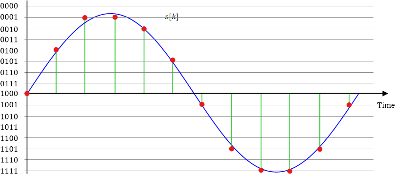
\] - On the other hand, an Analog to Digital Converter (ADC) works on the number of bits used to represent one signal level.

For example, the dynamic range of a 14-bit ADC with a voltage range from 0 to 5 V is computed as follows.
The highest level represents 5 V while the lowest level would represent a voltage of
\[
\frac{5}{2^{14}} = 0.0003 ~\text{V}
\]The dynamic range of this ADC is thus
\[
20 \log_{10} \frac{5}{0.0003} \approx 84 ~\text{dB}
\]

Modern electronic components frequently have a dynamic range of more than 100 dB, i.e.,
\[
10^{100/20} = 100,000
\]
This is quite a large number. For instance, this is the ratio between the distances from earth to sun as compared to that from Dallas to Chicago!
Noise Floor
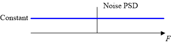
When no signal is present, the receiver voltage is not exactly zero as the electrons are not standing still. In any device, these electrons move around in a random fashion even in the absence of external signals. These random vibrations create a noise signal with an average value of zero. Due to this randomness, its Power Spectral Density (PSD) is constant for all frequencies ranging from $-\infty$ to $+\infty$, as shown in Figure below.
Since the motion of electrons produces a certain amount of heat, the noise generated by such a movement is called thermal noise. Nyquist investigated the properties of thermal noise and showed that its power spectral density is equal to
\[
\text{Noise Power Density} = k T~\text{W/Hz}
\]
where $k$ is the Boltzmann’s constant ($1.38\times 10^{-23}$ J/K) and $T$ is the temperature in Kelvin. In words, the noise power is directly proportional to the equivalent temperature at the receiver frontend.
At room temperature $290$ K, this becomes
\[
1.38\times 10^{-23} ~\times~ 290 = 4\times 10^{-21} ~\text{W/Hz}
\]
In terms of dBm, this quantity can be written as
\[
\text{Noise Power Density} = 10\log_{10}\frac{4\times 10^{-21}}{1~\text{mW}}/\text{Hz} = -174~\text{dBm/Hz}
\]
In summary, noise floor is the voltage level that is generated by nature through all the processes running in the background.
Sensitivity
Now we turn towards the minimum signal level to ensure proper demodulation. Starting from the background noise power density of $-174$ dBm above, the actual noise power entering the calculations depends on several factors.
- Bandwidth – Remember that the units of power density are in W/Hz. For a system bandwidth $B$, the noise power is given by the product between the spectral density and this bandwidth. This becomes an addition in a logarithmic relation.
\[
S = -174 + 10\log_{10}B \quad~\text{dBm}
\] - Noise Figure – Internally generated noise of the receiver components are quantified by Noise Figure (NF) given in dB. This needs to be added to the power budget.
\[
S = -174 + 10\log_{10}B + NF \quad~\text{dBm}
\] - Minimum Required SNR – The minimum required SNR (in dB) for signal detection or demodulation appears over and above the value computed so far.
\[
S = -174 + 10\log_{10}B + NF + SNR \quad~\text{dBm}
\]
A good measure of receiver sensitivity is SINAD in analog communication systems and Bit Error Rate (BER) in digital communication systems.
Example
As an example, the sensitivity of a receiver at room temperature for a bandwidth $B=1$ MHz (i.e., $10^6$ Hz), a noise figure of $10$ dB and a minimum required SNR of $15$ dB can be computed as follows.
\[
S = -174 + 60 + 10 + 15 = -89~\text{dBm}
\]
References
[1] R. Sobot, Wireless Communication Electronics – Introduction to RF Circuits and Design Techniques, Springer, 2012.