In case of Quadrature Amplitude Modulation (QAM) and other passband modulation schemes, Rx has no information about carrier phase of the Tx oscillator. Let us explore what impact this has on the demodulation process.
Constellation Rotation
To see the effect of the carrier phase offset, consider that a transmitted passband signal consists of two PAM waveforms in $I$ and $Q$ arms denoted by $v_I(t)$ and $v_Q(t)$ respectively and combined as
\begin{equation}\label{eqRealWorldQAMPhaseOffset}
s(t) = v_I(t) \sqrt{2} \cos 2\pi F_C t – v_Q(t) \sqrt{2}\sin 2\pi F_C t
\end{equation}
Here, $F_C$ is the carrier frequency and $v_I(t)$ and $v_Q(t)$ are the continuous versions of sampled signals $v_I(nT_S)$ and $v_Q(nT_S)$ given by
\begin{equation}
\begin{aligned}\label{eqRealWorldvIvQ}
v_I(nT_S)\: &= \sum _{i} a_I[i] p(nT_S-iT_M) \\
v_Q(nT_S) &= \sum _{i} a_Q[i] p(nT_S-iT_M)
\end{aligned}
\end{equation}
In the above equation, $a_I[m]$ and $a_Q[m]$ are the inphase and quadrature components of the $m^{th}$ symbol, $p(nT_S)$ are the samples of a square-root Nyquist pulse with support $-LG \le n \le LG$ and $T_S$ and $T_M$ are the sample time and symbol time, respectively.
In the absence of noise, the received signal for a passband waveform is the same as the transmitted signal except a carrier phase mismatch, i.e., we ignore every other distortion in the received signal except the phase offset $\theta_\Delta$.
After bandlimiting the incoming signal through a bandpass filter, it is sampled by the ADC operating at $F_S=1/T_S$ samples/second to produce
\begin{align*}
r(nT_S) &= v_I(nT_S) \sqrt{2}\cos \left(2\pi F_C nT_S + \theta_{\Delta}\right) – v_Q(nT_S)\sqrt{2} \sin\left( 2\pi F_C nT_S + \theta_{\Delta}\right) \\
&= v_I(nT_S) \sqrt{2}\cos \left(2\pi \frac{k_C}{N}n + \theta_{\Delta}\right) – v_Q(nT_S) \sqrt{2}\sin \left(2\pi \frac{k_C}{N}n + \theta_{\Delta}\right)
\end{align*}
where the relation $F/F_S = k/N$ is used and $k_C$ corresponds to $F_C$, and the angle $\theta_{\Delta}$ is the phase difference between the incoming carrier and the local oscillator at the Rx.
To produce a complex baseband signal from the received signal, the samples of this waveform are input to a mixer which multiplies them with discrete-time quadrature sinusoids $\sqrt{2}\cos 2\pi (k_C/N)n$ in the $I$ arm and $-\sqrt{2}$ $\cdot$ $\sin 2\pi (k_C/N)n$ for $Q$ arm. We continue the derivation for $I$ part and the same for $Q$ is very similar and the reader can solve it as an exercise. Using the identities $\cos(A)\cos(B)$ $= 0.5$ $\left( \cos(A+B)\right.\}$ $+$ $\left.\cos(A-B) \right)$ and $\sin(A)\cos(B)$ $= 0.5$ $\left( \sin(A+B)\right.\}$ $+$ $\left.\sin(A-B) \right)$,
\begin{equation*}
\begin{aligned}
x_I(nT_S) &= r(nT_S) \cdot \sqrt{2}\cos 2\pi \frac{k_C}{N}n \: \\
&= v_I(nT_S)\left\{\cos\theta_{\Delta} + \underbrace{\cos \left(2\pi \frac{2k_C}{N}n + \theta_{\Delta}\right)}_{\text{Double frequency term}} \right\} – \\
& \qquad \qquad \quad v_Q(nT_S) \left\{\sin \theta_{\Delta} + \underbrace{\sin \left(2\pi \frac{2k_C}{N}n + \theta_{\Delta} \right)}_{\text{Double frequency term}} \right\}
\end{aligned}
\end{equation*}
The matched filter output is written as
\begin{equation*}
\begin{aligned}
z_I(nT_S) &= x_I(nT_S) * p(-nT_S) \\
&= \left(v_I(nT_S) \cos \theta_{\Delta} – v_Q(nT_S) \sin\theta_{\Delta} + \right. \\
&\hspace{.6in}\left.\text{Double frequency terms}\right)* p(-nT_S)
\end{aligned}
\end{equation*}
The double frequency terms in the above equation are filtered out by the matched filter $h(nT_S) = p(-nT_S)$, which also acts a lowpass filter due to its spectrum limitation in the range $-0.5 R_M \le F \le +0.5R_M$, where $R_M$ is the symbol rate. Writing the definitions of $v_I(nT_S)$ and $v_Q(nT_S)$,
\begin{equation*}
\begin{aligned}
z_I(nT_S) = \sum_i \Big\{ a_I[i]\cos \theta_{\Delta} – a_Q[i]\sin\theta_{\Delta} \Big\} r_p(iT_M – nT_S)
\end{aligned}
\end{equation*}
where $r_p(nT_S)$ comes into play from the definition of auto-correlation function. To generate symbol decisions, $T_M$-spaced samples of the matched filter output are required at $n = mL = mT_M/T_S$. Downsampling the matched filter output generates
\begin{equation*}
\begin{aligned}
z_I(mT_M) &= z_I(nT_S) \bigg| _{n = mL = mT_M/T_S} \\
&= \sum \limits _i \Big\{ a_I[i]\cos \theta_{\Delta} – a_Q[i]\sin \theta_{\Delta}\Big\} r_p(iT_M – mT_M)
\end{aligned}
\end{equation*}
For a square-root Nyquist that satisfies no-ISI criterion, $r_p(iT_M – mT_M)$ is zero except for $i = m$. Thus,
\begin{equation*}
\begin{aligned}
z_I(mT_M) = a_I[m] \cos \theta_{\Delta} – a_Q[m]\sin\theta_{\Delta}
\end{aligned}
\end{equation*}
A similar derivation for $Q$ arm yields the final expression for the symbol-spaced samples in the presence of phase offset $\theta_{\Delta}$.
\begin{aligned}\label{eqRealWorldPhaseRotationIQ}
z_I(mT_M) = a_I[m] \cos \theta_{\Delta} – a_Q[m]\sin\theta_{\Delta} \\
z_Q(mT_M) = a_I[m] \sin \theta_{\Delta} + a_Q[m]\cos\theta_{\Delta}
\end{aligned}
\end{equation}
From the phase rotation rule of complex numbers, we know that this expression is nothing but counterclockwise rotation by an angle $\theta_{\Delta}$. In polar form, this expression can be written as
\begin{aligned}\label{eqRealWorldPhaseRotationMP}
|z(mT_M)| &= \sqrt{a_I^2[m] + a_Q^2[m]} \\
\measuredangle z(mT_M) &= \measuredangle \Big(a_Q[m],a_I[m]\Big) + \theta_{\Delta}
\end{aligned}
\end{equation}
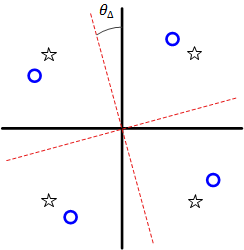
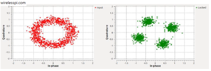
In conclusion, a mismatch of $\theta_{\Delta}$ between incoming carrier and Rx oscillator rotates the desired outputs $a_I[m]$ and $a_Q[m]$ on the constellation plane by an angle $\theta_{\Delta}$. This is drawn in the scatter plot of Figure below for a $4$-QAM constellation. Keep in mind that the blue circles are not one but several symbols mapped over one another due to the similar phase shift.
Cross-talk
Start with $\theta_{\Delta}=0$ and observe that the $I$ and $Q$ outputs are $a_I[m]$ and $a_Q[m]$, respectively. This implies that signals in $I$ and $Q$ arms are completely independent of each other. Gradually increasing $\theta_{\Delta}$ has two effects:
- Since $\cos \theta_{\Delta} < \cos 0 = 1$, amplitude of $a_I[m]$ in $z_I(mT_M)$ reduces. The same phenomenon happens with $a_Q[m]$ in $z_Q(mT_M)$.
- Since $\sin \theta_{\Delta} > \sin 0 = 0$, interference of $a_Q[m]$ in $z_I(mT_M)$ increases as well as that of $a_I[m]$ in $z_Q(mT_M)$.
This interference between $I$ and $Q$ components is known as cross-talk. Cross-talk increases with $\theta_{\Delta}$ until for a $90^\circ$ difference, $a_I[m]$ appears at $Q$ output and $-a_Q[m]$ at $I$ output.
The effect of this cross-talk on a Raised Cosine shaped $4$-QAM waveform with excess bandwidth $\alpha=0.5$ is shown in Figure below for a phase difference $\theta_{\Delta} = 30^\circ$. Observe the first sample: it is $(-1,+1)$ in quadrant II. After phase rotation, $I$ part moved towards left thus increasing its amplitude and $Q$ moved downwards reducing its amplitude. This is evident through the first samples in the Figure. A similar argument holds for all other symbols.
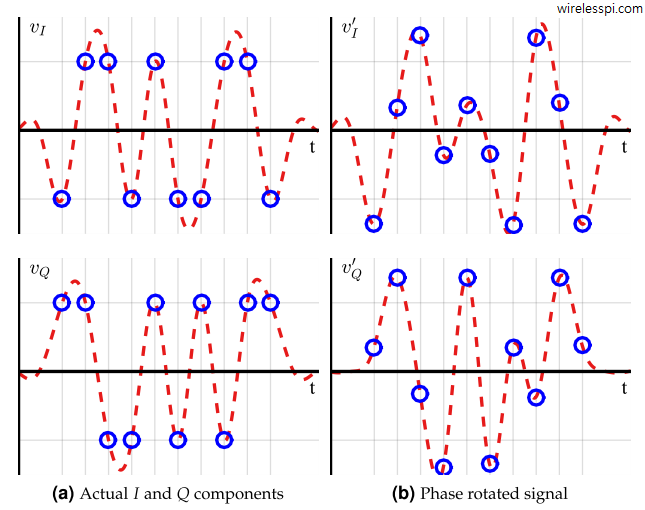
Something really interesting has happened in Figure above. Notice that although the amplitude has decreased for some symbols, it has risen for some other symbols as well. This is the outcome of a circular rotation. While it is good to have some symbols with a little extra protection against noise, remember that it has come at a cost of reduced amplitudes for other symbols, making them much vulnerable to noise and other impairments. The overall effect is negative, just like strengthening your right arm in exchange of significantly weakening the left is dangerous for your body.
Scatter Plot
What was discussed above can be extended to the whole symbol stream. The cumulative effect of a phase offset is straightforward to see in a scatter plot. There will be clouds of samples from downsampled matched filter output around the original constellation.
Eye Diagram
Since the scatter plot is different than a raw time domain waveform, we employ the eye diagram to examine the effects of carrier phase offset (say, on an oscilloscope). First, start with a BPSK modulation scheme and remember that there is no $Q$ channel in this case and consequently no cross-talk. However, the effect of phase rotation is a reduction in signal amplitude which can be observed by focusing on $I$ arm.
\begin{equation}
\begin{aligned}\label{eqRealWorldBPSKPhaseRotation}
z_I(mT_M) = a_I[m] \cos \theta_{\Delta}
\end{aligned}
\end{equation}
Since $\cos \theta_\Delta$ always lies between $-1$ and $1$, the amplitude of the $I$ signal gets reduced accordingly with the rest of the energy rising in the $Q$ arm. This signal is written as
\begin{equation*}
\begin{aligned}
z_Q(mT_M) = a_I[m] \sin \theta_{\Delta}
\end{aligned}
\end{equation*}
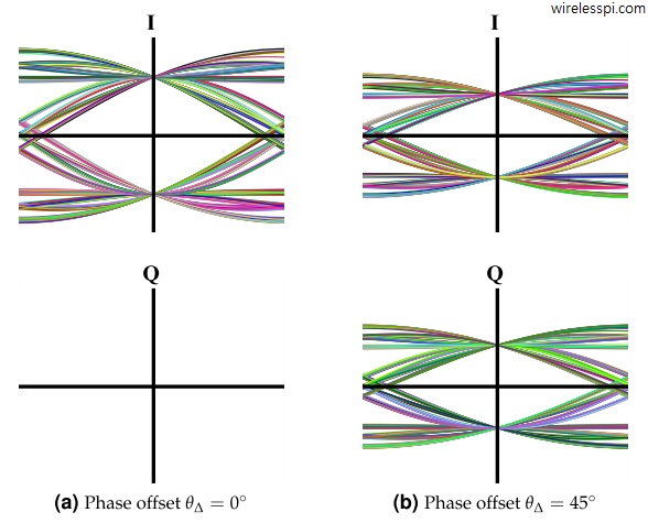
With a phase offset of $45^\circ$, the $I$ branch loses half of its energy with the remaining half going in the $Q$ arm. This is drawn in Figure below. In fact for a $90^\circ$ phase rotation, the $I$ contribution actually reaches zero and all the energy of the signal appears across the $Q$ branch. Due to this reason, we will see later that the $Q$ arm is still employed for BPSK signals — not for data detection but helping in the phase synchronization procedure.
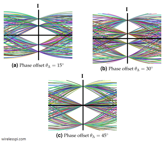
Next, we turn our focus towards QAM and observe the amplitude change and cross-talk between $I$ and $Q$ branches for three different phase offsets, $15^{\circ}$, $30^{\circ}$ and $45^{\circ}$. Figure below illustrates the $I$ channel for these phase offsets in a noiseless case and a $4$-QAM signal. A similar diagram holds for $Q$ arm as well and not drawn here. The optimal sampling instants are still visible due to zero noise but \bbf{the eye diagram looks more like a $4$-PAM signal than that of a single $4$-QAM signal due to the cross-talk from $Q$ arm}. It is also evident that $I$ and $Q$ affect each other in equal proportions.

The reason there are only two eyes for $45^\circ$ phase offset is that $\cos \theta_\Delta$ and $\sin \theta_\Delta$ become equal and hence many symbols $a_I$ and $a_Q$ cancel each in both $I$ and $Q$ arms of the output. In terms of the scatter plot, a rotation of $45^\circ$ shifts the constellation points onto the real and imaginary axes, so for the $I$ plot shown here, the output at the sampling instant coincides only with a positive or negative symbol value.
Concluding Remarks
- Carrier phase synchronization can be accomplished through a Phase Locked Loop (PLL) that is a feedback solution. Feedforward strategies estimate and compensate for the phase once and for all, see this conjugate product phase estimator as an example.
- Other techniques to acquire phase are also available, e.g., the popular M-th power synchronizer in both feedback and feedforward settings.
Hello,
I am trying to understand effect of CFO on OFDM system. When we consider an OFDM system, we have multiple s(t) signals right? Each of these signals will have the same phase rotation?
What exactly do you mean by multiple s(t) signals? Please have a look at my article on OFDM. From here, we can conclude that the effect of Carrier Frequency Offset (CFO) is to ‘sample’ the discrete bins at non-peak values. Just like a signal is sampled in time domain at the peak to avoid Inter-Symbol Interference (ISI), a CFO in an OFDM signal accesses the subcarriers at non-optimal positions and introduces Inter-Carrier Interference (ICI).