Quadrature Amplitude Modulation (QAM) is a spectrally efficient modulation scheme used in most of the high-speed wireless networks today. We discussed earlier that Pulse Amplitude Modulation (PAM) transmits information through amplitude scaling of the pulse $p(nT_S)$ according to the symbol value. To understand QAM, two routes need to be traversed.
Route 1
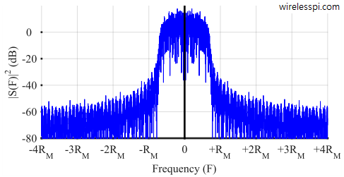
We start the first route with differentiating between baseband and passband signals. A baseband signal has a spectral magnitude that is nonzero only for frequencies around origin ($F=0$) and negligible elsewhere. An example spectral plot for a PAM waveform is shown below for 500 2-PAM symbols shaped by a Square-Root Raised Cosine pulse with excess bandwidth $\alpha = 0.5$ and samples/symbol $L = 8$. The PAM signal has its spectral contents around zero and hence it is a baseband signal.
For wireless transmission, this information must be transmitted through space as an electromagnetic wave. Also observe that once this spectrum is occupied, no other entity in the surrounding region can share the wireless channel for the purpose of communications. For these reasons (and a few others as well), a wireless system is allocated a certain bandwidth around a higher carrier frequency and the generated baseband signal is shifted to that specific portion of the spectrum. Such signals are called passband signals. That is why wireless signals in everyday use such FM radio, WiFi, cellular like 4G, 5G, and Bluetooth are all passband signals which execute their transmissions within their respective frequency bands sharing the same physical medium.
The easiest method to shift the spectrum to a designated carrier frequency is by multiplying, or mixing, it with a sinusoidal waveform due to the following reason.
- In time domain, a PAM waveform can be multiplied with a carrier sinusoid at frequency $F_C$.
- Time domain multiplication between two signals is frequency domain convolution between their spectra.
- The spectrum of a pure sinusoid at any frequency is composed of two impulses at that frequency (one positive and one negative, both with half the amplitude).
- Hence in frequency domain, the convolution of a signal with a unit impulse results in the same signal “parked” at its allocated slot.
This is drawn in the figure below.
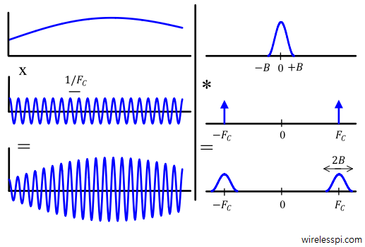
After this spectral upconversion, both positive and negative portions of the baseband spectrum appear at $+F_C$ and $-F_C$. The bandwidth — positive portion of the spectrum — hence becomes double. However, a relief comes from the fact that both $\cos(\cdot)$ and $\sin (\cdot)$ can be used to carry independent waveforms due to their orthogonality (having phases $90 ^\circ$ apart) to each other over a complete period, i.e.,
\begin{equation*}
\sum \limits _{n=0} ^{N-1} \cos 2\pi \frac{k}{N}n \cdot \sin 2\pi \frac{k}{N}n = 0
\end{equation*}
Obviously, this is true over a complete period. However, this is approximately true for very high carrier frequencies (typical case in wireless communications) as well because $2\cos A \sin A = \sin 2A$ that doubles the frequency. Due to positive and negative halves of a sine, the area under the curve (sum of samples) is then zero for all integer number of cycles. This area under any fraction of a cycle outside the last integer cycle then remains negligible at a high carrier frequency.
Route 2
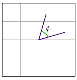
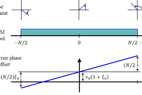
The second route starts with amplitude modulation, where all the amplitudes still extend on the same axis of the PAM constellation diagram. On the other hand, for a phase modulated system, one axis is not enough because an actual angle is formed by two lines, not one. This is shown in the figure below. In other words, an amplitude modulation scheme has a 1-dimensional constellation diagram while a phase modulation scheme requires a 2-dimensional constellation diagram.
If amplitude modulation sends the information on discrete amplitudes in one dimension and phase modulation chooses a set of discrete phases in two dimensions but on the same circle, both of these ideas can be combined together in the form of Quadrature Amplitude Modulation (QAM). For a practical implementation of this idea, we start with introducing both amplitude and phase modulation in a carrier waveform.
\begin{equation}\label{equation-qam}
s(t) = A_m\cdot \cos \left(2\pi Ft + \phi_m\right)
\end{equation}
Using the identity $\cos (A+B)$ $=$ $\cos A \cos B$ $-$ $\sin A \sin B$, we open this up as
\begin{equation}\label{equation-qam-iq}
\begin{aligned}
s(t) &= A_m\cdot \cos (2\pi Ft)\cdot \cos \phi_m – A_m \cdot \sin 2\pi Ft \cdot \sin \phi_m \\
&= \underbrace{(A_m\cos \phi_m)}_{\text{I part}}\cdot \cos (2\pi Ft) – \underbrace{(A_m \sin \phi_m)}_{\text{Q part}} \cdot \sin 2\pi Ft
\end{aligned}
\end{equation}
Here, the amplitude $A_m\cos \phi_m$ is the projection of the modulation point on $x$ axis, while the amplitude $A_m\sin \phi_m$ is the projection of the modulation point on $y$ axis. This is plotted in the figure below. These amplitudes are then modulated on two quadrature carriers, namely $\cos (2\pi Ft)$ and $-\sin (2\pi Ft)$ and summed together to be sent over the air. Why are there two waveforms as opposed to one (before the summation)? Because constructing or measuring an angle requires two lines, and hence constructing or measuring a phase requires two waveforms, one for each line.
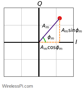
To explain $I$ and $Q$ notations further, recall that each phase, like each angle, needs a reference. For an angle, this reference is provided by the horizontal line connecting point $(0,0)$ to point $(1,0)$. For a phase, a cosine wave with phase $0^\circ$, i.e., $\cos (2\pi Ft)$, is taken as the reference (an arbitrary choice). Acting as an amplitude of this waveform $\cos (2\pi Ft)$, the symbol level $A_m\cos \phi_m$ on the horizontal axis is known as the In-Phase component (in phase with a cosine), from which the notation $I$ is extracted.
To understand the $Q$ part, we need another waveform to represent the amplitude on the vertical axis. If the horizontal axis links angle $0^\circ$ on a 2-D plane to a cosine wave $\cos (2\pi Ft)$ with the starting phase $0^\circ$, then the vertical axis at an angle $90^\circ$ on a 2-D plane should be linked to which waveform? Clearly, this should be another cosine wave with the starting phase of $90^\circ$. A cosine wave with a starting phase of $90^\circ$ is found by
\begin{equation*}
\cos \left (2\pi F t + 90^\circ\right) = \cos 2\pi F t \cdot \underbrace{\cos 90^\circ}_{0} – \sin 2\pi Ft\cdot \underbrace{\sin 90^\circ}_{1} = – \sin 2\pi Ft
\end{equation*}
This second cosine wave comes out to be a negative sine wave!
That is the birth of Quadrature Amplitude Modulation (QAM), in which two independent PAM waveforms are communicated through mixing one with a cosine and the other with a sine. Just like constellation, the term quadrature also comes from astronomy to describe position of two objects $90 ^\circ$ apart. An interested reader can see the following articles on I/Q signals for further details.
- Two birds with one tone: I/Q signals and Fourier Transform.
- IQ signals 101 – Neither complex nor complicated.
Mathematical Expression
For mathematical expression for QAM, first consider two independent PAM waveforms with symbol streams $a_I$ and $a_Q$, respectively.
$$\begin{equation}
\begin{aligned}
v_I(nT_S)\: &= \sum _{m} a_I[m] p(nT_S-mT_M) \\
v_Q(nT_S) &= \sum _{m} a_Q[m] p(nT_S-mT_M)
\end{aligned}
\end{equation}\label{eqCommSystemQAMarms}$$
Next, we multiply the resulting complex signal with a complex sinusoid at carrier frequency and collect its real part, i.e., multiply $v_I$ arm with $\sqrt{2}\cos 2\pi (k_C/N) n$ and $v_Q$ arm with $-\sqrt{2}\sin 2\pi (k_C/N) n$. The reason of including these two factors, $\sqrt{2}$ and the negative sign, will be discussed later during QAM detection. Consequently, a general QAM waveform can be written as
\begin{align}
s(nT_S) &= v_I(nT_S) \sqrt{2} \cos 2\pi \frac{k_C}{N} n – v_Q(nT_S) \sqrt{2}\sin 2\pi \frac{k_C}{N} n \label{eqCommSystemQAMWaveformDiscrete} \\
&= v_I(nT_S) \sqrt{2}\cos 2\pi \frac{F_C}{F_S}n – v_Q(nT_S) \sqrt{2}\sin 2\pi \frac{F_C}{F_S}n \nonumber
\end{align}
\begin{align}
&= \sum _{m} a_I[m] p(nT_S-mT_M) \sqrt{2}\cos 2\pi F_C nT_S – \nonumber \\
&~ \hspace{1in} \sum _{m} a_Q[m] p(nT_S-mT_M) \sqrt{2}\sin 2\pi F_C nT_S \nonumber
\end{align}
where we have used the fundamental relation between continuous and discrete frequencies $k/N = F/F_S$, and $k_C$ corresponds to the carrier frequency $F_C$. Observe that $s(nT_S)$ is a real signal with no $Q$ component. After digital to analog conversion (DAC), the continuous-time signal $s(t)$ can be expressed as
\begin{align}
s(t) &= v_I(t) \sqrt{2} \cos 2\pi F_C t – v_Q(t) \sqrt{2}\sin 2\pi F_C t \label{eqCommSystemQAMWaveformContinuous} \\
&= \sum _{m} a_I[m] p(t-mT_M)\sqrt{2} \cos 2\pi F_C t ~- \nonumber \\
&~ \hspace{1in} \sum _{m} a_Q[m] p(t-mT_M) \sqrt{2} \sin 2\pi F_C t \nonumber
\end{align}
In Eq \eqref{eqCommSystemQAMWaveformContinuous}, symbols $a_I[m]$ determine the $I$ signal while $a_Q[m]$ control the $Q$ signal. Such representation of the QAM waveform as a sum of amplitude scaled and pulse shaped sinusoids is known as the rectangular form. Using trigonometric identity $\cos (A+B) = \cos A \cos B – \sin A \sin B$, Eq \eqref{eqCommSystemQAMWaveformContinuous} can also be written as
\begin{equation*}
s(t) = \sqrt{a_I^2[m] + a_Q^2[m]} \cdot p(t-mT_M) \cdot \sqrt{2} \cos \left(2\pi F_C t+ \tan^{-1} \frac{a_Q[m]}{a_I[m]}\right)
\end{equation*}
Called the polar form, here we have a single sinusoid whose amplitude and phase are determined by some combination of symbols $a_I[m]$ and $a_Q[m]$.
Constellation Diagram
Some examples of QAM constellations are discussed below.
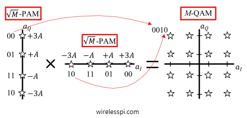
- For an even power of $2$, square QAM is a constellation whose points are spaced on a grid in the form of a square. It is formed by a product of two $\sqrt{M}$-PAM constellations, one on $I$ axis and the other on $Q$ axis. For example, a $16$-QAM constellation is formed by two $\sqrt{16}=4$ PAM constellations as drawn in Figure below, while some other square QAM constellations are also shown in the next figure.
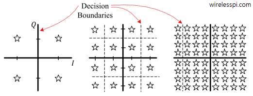
Notice how constellation points in higher-order QAM are closer to each other compared to lower-order QAM. A relatively lower noise power is then enough to cause a decision error by moving the received symbol over the decision boundary. This is the cost of increasing data rate by packing more bits in the same symbol. We will have more to say about it when we discuss Bit Error Rates (BER) for each constellation in another article.
For $M=4$, the average symbol energy in square QAM is derived using Pythagoras theorem as
\begin{equation*}
E_{4-\text{QAM}} = \frac{1}{4}\left\{ 4 \left( A^2 + A^2\right) \right\} = 2A^2
\end{equation*}
For general $M$, a similar derivation as in the case of PAM yields
\begin{equation}\label{eqCommSystemQAMEnergy}
E_{M-\text{QAM}} = \frac{2}{3} \left(M-1\right)A^2
\end{equation} - A special case of $M$-QAM is $M$-PSK, which stands for Phase Shift Keying. As the name PSK implies, the amplitude remains constant in this configuration while the information is conveyed by different phases. Examples of $2$-PSK, $4$-PSK and $8$-PSK are drawn in Figure below.
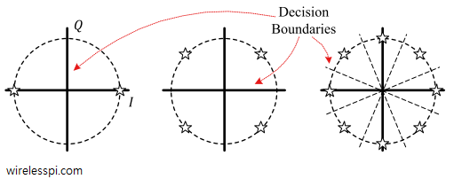
Notice that
- $2$-PSK constellation (also known as BPSK) looks similar to $2$-PAM. However, the difference is that there is no carrier upconversion in PAM systems.
- $4$-PSK constellation (also known as QPSK) is exactly the same as square $4$-QAM.
- For $M>4$, square QAM packs the constellation points more efficiently than $PSK$ and hence the modulation of choice in many wireless standards. Points come relatively closer in PSK and the closer the points, the larger the probability of receiving a symbol in error due to a jump across the decision boundary. On the other hand, QAM heavily depends on overall system linearity due to information conveyed in the signal amplitude. A constant envelope of the modulated signal is much more suitable for transmission over nonlinear channels where PSK is the preferred choice. In such situations, the performance of PSK is quite insensitive to nonlinear distortion and heavy filtering.
- Since any constellation that uses both amplitude and phase modulation fall under the general category of QAM, there can be many other rearrangements of QAM constellation points. However, we focus on square QAM and PSK in this text which are widely used in practice. Non-regular constellations can be formed which yield a small performance advantage, though it is usually not much significant. Moreover, the more points are in the constellation, the lesser is the difference.


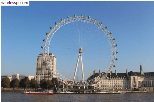
Here is a little quiz for you: which PSK constellation is the London Eye shown in Figure below? The answer is $32$-PSK as the Eye has $32$ pods but they are numbered from $1$ to $33$. The number $13$ is skipped for keeping the luck on our side.
QAM Modulator
To build a conceptual QAM modulator, we follow similar steps as in a PAM modulator. The block diagram for a $4$-QAM modulator is drawn in Figure below.
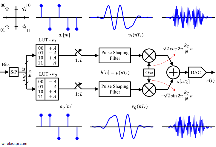
- Every $T_b$ seconds, a new bit arrives at the input forming a serial bit stream.
- A serial-to-parallel (S/P) converter collects $\log_2 M$ such bits every $T_M = \log_2 M \times T_b$ seconds that are used as an address to access two Look-Up Tables (LUT). One LUT stores $\sqrt{M}$ symbol values $a_I$ while the other $\sqrt{M}$ symbol values $a_Q$ specified by the constellation.
- To produce a QAM waveform, the symbol sequences $a_I[m]$ and $a_Q[m]$ are converted to discrete-time impulse trains in separate arms (one $I$ and the other $Q$) through upsampling by $L$, where $L$ is samples/symbol defined in as ratio of symbol time to sample time $T_M/T_S$, or equivalently sample rate to symbol rate $F_S/R_M$.
- As explained in sample rate conversion, upsampling inserts $L-1$ zeros between each symbol after which the interpolated intermediate samples can be raised from dead with the help of a pulse shaping filter in each arm that — in addition to shaping the spectrum — suppresses all the spectral replicas arising from upsampling except the primary one. These are the two $I$ and $Q$ PAM waveforms forming the signal $v_I$.
- Next, $I$ PAM waveform $v_I$ is upconverted by mixing with the carrier $\cos 2\pi F_C nT_S$ while the $Q$ PAM waveform $v_Q$ with $-\sin 2\pi F_C nT_S$, which are then summed to form the QAM signal $s(nT_S)$. The carriers are generated through an oscillator at the Tx.
- This discrete-time signal $s(nT_S)$ is converted to a continuous-time signal $s(t)$ by a DAC.
The mathematical derivation for the QAM modulator was shown in Eq \eqref{eqCommSystemQAMWaveformDiscrete} and Eq \eqref{eqCommSystemQAMWaveformContinuous}.
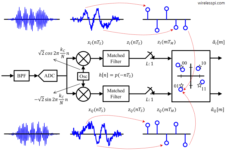
QAM Detector
The received signal $r(t)$ is the same as the transmitted signal $s(t)$ but with the addition of additive white Gaussian noise (AWGN) $w(t)$. The symbols are detected through the following steps illustrated in Figure below.

- Out of the infinite spectrum, the desired signal $r(t)$ is selected with the help of a Bandpass Filter (BPF).
- Through an analog to digital converter (ADC), this signal is sampled at a rate of $F_S$ samples/s to produce a sequence of $T_S$-spaced samples $r(nT_S)$.
- Next, a complex signal $x(nT_S$ is produced when $r(nT_S)$ by downconverted by mixing with two carriers, $\cos 2\pi F_C nT_S$ and $\sin 2\pi F_C nT_S$ which are generated through an oscillator at the Rx.
- The resulting complex waveform $x(nT_S)$ in $I$ and $Q$ arms is processed through two matched filters thus generating $z_I(nT_S)$ and $z_Q(nT_S)$. As discussed earlier, the output of the matched filters are continuous correlations of the symbol-scaled pulse shape with an unscaled and time-reversed pulse shape.
- These $I$ and $Q$ outputs are downsampled by $L$ at optimal sampling instants
\begin{equation*}
n = mL = m \frac{T_M}{T_S}
\end{equation*}
to produce $T_M$-spaced numbers $z_I(mT_M)$ and $z_Q(mT_M)$ back from the signal. - The minimum distance decision rule is employed in $IQ$-plane to find the symbol estimates $\hat a_I[m]$ and $\hat a_Q[m]$ to decide on the final constellation point.
Let us discuss the mathematical details of this process for a noiseless received signal as in Eq \eqref{eqCommSystemQAMWaveformContinuous},
\begin{equation}\label{eqCommSystemRxQAMSignalNoiseless}
r(t) = s(t) = v_I(t) \sqrt{2} \cos 2\pi F_C t – v_Q(t) \sqrt{2}\sin 2\pi F_C t
\end{equation}
where $F_C$ is the carrier frequency and $v_I(t)$ and $v_Q(t)$ are defined in Eq \eqref{eqCommSystemQAMarms}. After bandlimiting the incoming signal through a bandpass filter, it is sampled by the ADC operating at $F_S$ samples/second to produce
\begin{align*}
r(nT_S) &= v_I(nT_S) \sqrt{2}\cos 2\pi F_C nT_S – v_Q(nT_S)\sqrt{2} \sin 2\pi F_C nT_S \\
&= v_I(nT_S) \sqrt{2}\cos 2\pi \frac{k_C}{N}n – v_Q(nT_S) \sqrt{2}\sin 2\pi \frac{k_C}{N}n
\end{align*}
where the relation $F/F_S = k/N$ is used. To produce a complex baseband signal from the received signal, the samples of this waveform are input to a mixer which multiplies them with discrete-time quadrature sinusoids $\sqrt{2}\cos 2\pi (k_C/N)n$ and $-\sqrt{2}\sin 2\pi (k_C/N)n$ yielding
\begin{align*}
\begin{aligned}
x_I(nT_S) &= r(nT_S) \cdot \sqrt{2}\cos 2\pi \frac{k_C}{N}n \: \\
&= 2v_I(nT_S) \cos^2 2\pi \frac{k_C}{N}n – 2v_Q(nT_S) \sin 2\pi \frac{k_C}{N}n \cos 2\pi \frac{k_C}{N}n
\end{aligned}
\end{align*}
\begin{align*}
\begin{aligned}
x_Q(nT_S) &= r(nT_S) \cdot -\sqrt{2}\sin 2\pi \frac{k_C}{N} n \\
&= 2v_Q(nT_S) \sin ^2 2\pi \frac{k_C}{N}n -2v_I(nT_S) \cos 2\pi \frac{k_C}{N}n \sin 2\pi \frac{k_C}{N}n
\end{aligned}
\end{align*}
Using the identities $\cos^2 A = 1/2(1+\cos 2A)$, $\sin^2 A = 1/2(1-\cos 2A)$ and $2 \sin A \cos A = \sin 2A$,
\begin{align*}
\begin{aligned}
x_I(nT_S) &= v_I(nT_S) + \underbrace{v_I(nT_S)\cos 2 \pi \frac{2k_C}{N}n – v_Q(nT_S) \sin 2\pi \frac{2k_C}{N}n}_{\text{Double frequency terms}} \\
x_Q(nT_S) &= v_Q(nT_S) – \underbrace{v_Q(nT_S)\cos 2\pi \frac{2k_C}{N}n – v_I(nT_S) \sin 2\pi \frac{2k_C}{N}n}_{\text{Double frequency terms}}
\end{aligned}
\end{align*}
Now we can observe why the two factors, a $\sqrt{2}$ with both sinusoids and a negative sign with $\sin 2\pi (k/N)n$, were inserted.
- A $\sqrt{2}$ at the modulator and later another $\sqrt{2}$ in the detector result in a gain of $2$, which cancels the halving of sinusoid amplitudes in above trigonometric multiplications.
- When a complex signal is multiplied with a complex sinusoid, a negative sign appears for phase addition of $I$ and $Q$ in the $I$ section of cumulative waveform (from multiplication rule of complex numbers). This $I$ section of the cumulative waveform is the real part of the complex product which is transmitted through the channel. Another negative sign with $\sin 2\pi (k/N)n$ at the Rx delivers a positive $v_Q(nT_S)$ at the output.
The matched filter output is written as
\begin{align*}
\begin{aligned}
z_I(nT_S) &= x_I(nT_S) * p(-nT_S) \\
&= \left(v_I(nT_S) + \text{Double freq terms}\right) * p(-nT_S) \\
&= \Big( \sum \limits _i a_I[i] p(nT_S – iT_M) + \frac{2k_C}{N}~ \text{terms}\Big) * p(-nT_S) \\
&= \sum \limits _i a_I[i] r_p(nT_S – iT_M)
\end{aligned}
\end{align*}
\begin{align*}
\begin{aligned}
z_Q(nT_S) &= x_Q(nT_S) * p(-nT_S) \\
&= \left(v_Q(nT_S) + \text{Double freq terms}\right) * p(-nT_S) \\
&= \Big( \sum \limits _i a_Q[i] p(nT_S – iT_M) + \frac{2k_C}{N}~ \text{terms}\Big) * p(-nT_S) \\
&= \sum \limits _i a_Q[i] r_p(nT_S- iT_M)
\end{aligned}
\end{align*}
where $r_p(nT_S)$ comes into play from the definition of auto-correlation function. The double frequency terms in the above equation are filtered out by the matched filter $h(nT_S) = p(-nT_S)$, which also acts a lowpass filter due to its spectrum limitation in the range $-0.5 R_M \le F \le +0.5R_M$. To generate symbol decisions, $T_M$-spaced samples of the matched filter output are required at $n = mL = mT_M/T_S$. Downsampling the matched filter output generates
\begin{align*}
\begin{aligned}
z_I(mT_M) &= z_I(nT_S) \bigg| _{n = mL = mT_M/T_S} \\
&= \sum \limits _i a_I[i] r_p(mT_M – iT_M) = \sum \limits _i a_I[i] r_p\{(m-i)T_M\} \\
&= \underbrace{a_I[m] r_p(0T_M)}_{\text{current symbol}} + \underbrace{\sum \nolimits _{i \neq m} a_I[i] r_p\{(m-i)T_M\}}_{\text{ISI}}
\end{aligned}
\end{align*}
and
\begin{align*}
\begin{aligned}
z_Q(mT_M) &= z_Q(nT_S) \bigg| _{n = mL = mT_M/T_S} \\
&= \sum \limits _i a_Q[i] r_p(mT_M – iT_M) = \sum \limits _i a_Q[i] r_p\{(m-i)T_M\} \\
&= \underbrace{a_Q[m] r_p(0T_M)}_{\text{current symbol}} + \underbrace{\sum \nolimits _{i \neq m} a_Q[i] r_p\{(m-i)T_M\}}_{\text{ISI}}
\end{aligned}
\end{align*}
A square-root Nyquist pulse $p(nT_S)$ has an auto-correlation $r_p(nT_S)$ that satisfies no-ISI criterion,
\begin{equation*}
r_p(mT_M) = \left\{ \begin{array}{l}
1, \quad m = 0 \\
0, \quad m \neq 0 \\
\end{array} \right.
\end{equation*}
Thus,
\begin{align*}
\begin{aligned}
z_I(mT_M) &= a_I[m] \\
z_Q(mT_M) &= a_Q[m] \\
\end{aligned}
\end{align*}
In conclusion, the downsampled matched filter outputs map back to the Tx symbols in the absence of noise. If the world was simple, that would have been an end to it! But the world is complicated, and there are layers of issues that happen between the Tx information generation and Rx decision making. Anything we do after this will be to combat a subset of signal distortions and towards recovering the original information.
Observe that the system shown in Figure above is a multirate system. In the QAM detector, for example, the ADC and the matched filters operate at the sample rate $F_S$. After the outputs of the matched filters are downsampled by $L$, the symbol decisions are made at the symbol rate $R_M$. Furthermore, there are some hidden assumptions in the QAM detector:
[Symbol timing synchronization] The peak samples at the end of symbol durations in both $I$ and $Q$ arms are not known in advance at the Rx and in fact do not necessarily coincide with the generated samples as well. This is because ADC just samples the incoming continuous waveform without any information about the symbol boundaries. This is a symbol timing synchronization problem.
[Resampling] The ADC in general does not produce an integer number of samples per symbol, i.e., $T_M/T_S$ is not an integer. As we will see later, a resampling system is required in the Rx chain that changes the sample rate from the ADC rate to a rate that is an integer multiple of the symbol rate.
[Carrier frequency synchronization] The carrier frequency of the oscillator at the Tx and that at the Rx are not exactly the same. Instead, if the oscillator frequency at the Tx is denoted as $F_C$, then at the Rx, we have $F_C+F_\Delta$, where $F_\Delta$ is the difference between the two and can be either positive or negative. Any movement by the Tx, the Rx or within the environment between them also causes a shift in frequency (known as Doppler shift) that needs to be compensated.
[Carrier phase synchronization] Furthermore, the carrier phase at the Rx oscillators is not known beforehand and needs to be estimated.
[Equalization] Only an AWGN channel has been assumed so far. Multipath reflections from a wireless channel introduce ISI and distortion in the signal that need to be recovered through an equalizer.
QAM Eye Diagram and Scatter Plot
As discussed above, a QAM signal consists of two PAM signals riding on orthogonal carriers. At baseband, these two PAM signals appear as $I$ and $Q$ components of a complex signal at the Tx and Rx. Therefore, there are two eye diagrams for a QAM modulated signal, one for $I$ and the other for $Q$ and both of them are exactly the same as PAM.
The case of scatter plot is a little different. After downsampling the matched filter output to symbol rate, the samples thus obtained are mapped back to the constellation, previously illustrated in QAM detector block diagram and now drawn in Figure below for $4$-QAM modulation. This cloud of samples around the constellation points is now $2$-dimensional (for PAM, there was no $Q$ component) and can also be understood as a plot of $Q$ versus $I$ for each mapped value.
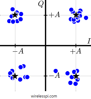
Looking at the scatter plot, one can readily deduce a lot of features for the particular transmission system. At this stage, however, it is enough to observe that the diameter of these clouds is a rough measure of the noise power corrupting the signal. For the ideal case of no noise, this diameter is zero and all the optimally timed samples coincide with their respective constellation points.
Finally, if you are further interested in learning about frequency modulation techniques instead of amplitude and phase, you can read the articles on analog FM and Frequency Shift Keying (FSK).

Hello Mr. Chaudhari
Can you comment or cover a topic on combining 2 QPSK modulator
to generate a 16QAM signal.
Thanks
Hi Bhudeb
In an SDR world, this is quite straightforward. Through a little modification, you can specify the output of the first modulator to indicate the quadrant and the output of the second modulator to indicate the symbol within that quadrant.
Just in case you are working on 16-QAM demodulators, then remember that a 16-QAM constellation can be treated as two QPSK modulations (one inner circle, one outer circle) plus one 8-PSK modulation (the middle circle).