In the article on modulation – from numbers to signals, we said that the Pulse Amplitude Modulation (PAM) is an amplitude scaling of the pulse $p(nT_S)$ according to the symbol value. What happens when this process of scaling the pulse amplitude by symbols is repeated for every symbol during each interval $T_M$? Clearly, a series of bits $b$ (1010 in our initial example) can be transmitted by choosing a rectangular pulse and scaling it with appropriate symbols.
\begin{equation*}
\begin{aligned}
m = 0 \quad b = 1 \quad a[0] = +A \\
m = 1 \quad b = 0 \quad a[1] = -A \\
m = 2 \quad b = 1 \quad a[2] = +A \\
m = 3 \quad b = 0 \quad a[3] = -A
\end{aligned}
\end{equation*}
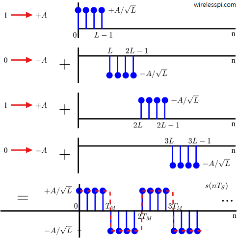
Our next step is forming a cumulative waveform from these individual symbol-scaled pulses. Remember from the article on transforming a signal that mathematical expression for a signal $p(nT_S)$ delayed by an amount $T_M$ or $L$ samples is given as $p(nT_S-LT_S)$ $=$ $p(nT_S-T_M)$, where $T_M$ is the symbol duration and $L$ is samples/symbol defined as $T_M/T_S$. Since the same pulse is scaled by the symbol value during each $T_M$,
- At time instant $0T_M$, the output is $a[0] p(nT_S-0T_M)$.
- At time instant $1T_M$, the output is $a[1] p(nT_S-1T_M)$.
- At time instant $2T_M$, the output is $a[2] p(nT_S-2T_M)$.
- At time instant $3T_M$, the output is $a[3] p(nT_S-3T_M)$.
And so on. Finally, their addition gives the expression for a general PAM waveform:\
\begin{equation}
\begin{aligned}\label{eqCommSystemPAMWaveformDiscrete}
s(nT_S) &= a[0]p(nT_S-0T_M) + a[1]p(nT_S-1T_M) + \\
& \hspace{1in} a[2] p(nT_S-2T_M) + a[3]p(nT_S-3T_M) + \cdots \\
&= \sum _{m} a[m] p(nT_S-mT_M)
\end{aligned}
\end{equation}
After digital to analog conversion (DAC), the continuous-time signal $s(t)$ can be expressed as
\begin{align}
s(t) &= \sum _{m} a[m] p(t-mT_M) \label{eqCommSystemPAMWaveformContinuous}
\end{align}
As an example, a $2$-PAM waveform is illustrated in Figure below with red dashed curve being the underlying continuous-time signal.
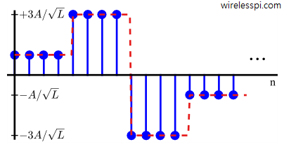
In a similar manner to $2$-PAM, a $4$-PAM waveform based on $4$ symbols can be constructed by scaling the pulse amplitude by different symbol values during each $T_M$, as illustrated in Figure below.
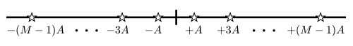
Constellation Diagram
Just like a constellation of stars, a constellation diagram shows the actual symbol values representing a set of $\log_2 M$ bits. We have already encountered constellation diagrams before (e.g., in the article on a simple communication system). A general constellation diagram for M-PAM is shown in Figure below.
Average Symbol Energy
The average symbol energy in a constellation is given by the average of all individual symbol energies. For $M=2$,
\begin{align*}
E_{M-\text{PAM}} &= \frac{A^2}{2}\left\{(+1)^2 + (-1)^2 \right\} = A^2
\end{align*}
And for $M=4$,
\begin{align*}
E_{M-\text{PAM}} &= \frac{A^2}{4}\left\{(-3)^2 + (-1)^2 + (+1)^2 + (+3)^2\right\} = 5A^2
\end{align*}
For a general $M$,
\begin{align*}
E_{M-\text{PAM}} &= \frac{A^2}{M}\left\{(-M+1)^2 + \cdots (-3)^2 + (-1)^2 + \right.\\
&~ \left. \hspace{2in} (+1)^2 + (+3)^2 + \cdots + (M-1)^2\right\} \\
&= 2\frac{A^2}{M}\left\{1^2 + 3^2 + \cdots + (M-1)^2\right\}
\end{align*}
The term in the brackets is the sum of squares of first $(M-1+1)/2$ $=$ $M/2$ odd integers. Using the formula $k(2k-1)(2k+1)/3$ for the first $k$ odd integers squared, we get
\begin{align}
E_{M-\text{PAM}} &= 2\frac{A^2}{M} \cdot \frac{M/2 \cdot (M-1) \cdot (M+1)}{3} \nonumber \\
&= \frac{M^2-1}{3} A^2 \label{eqCommSystemPAMEnergy}
\end{align}
The main purpose of this text is to find the answer to the following question: which operations are necessary to perform at the Tx and Rx sides such that we can detect that symbol with the highest probability? To explore the answer, we start with a simple PAM modulator and detector.
PAM Modulator
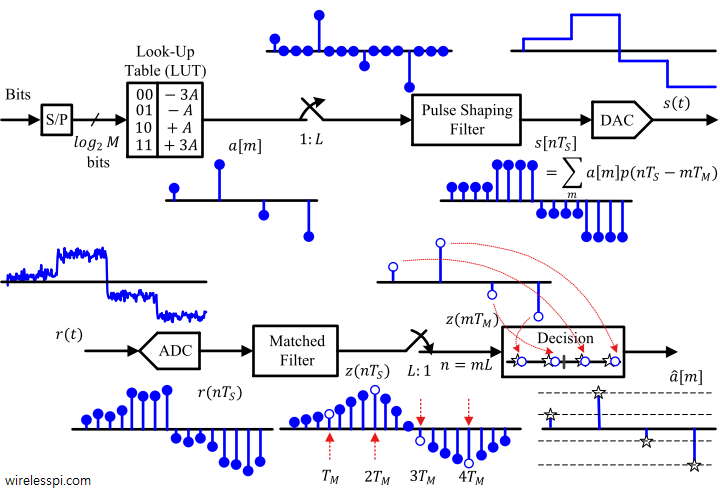
At this stage, we are ready to build a conceptual PAM modulator. The block diagram is drawn in Figure below in which Tx signal is generated in the following way.
- Every $T_b$ seconds, a new bit arrives at the input forming a serial bit stream.
- A serial-to-parallel (S/P) converter collects $\log_2 M$ such bits every $T_M = \log_2 M \times T_b$ seconds that are used as an address to access a Look-Up Table (LUT) that stores $M$ symbol values specified by the constellation.
- To produce a PAM waveform, the symbol sequence $a[m]$ is converted to a discrete-time impulse train through upsampling by $L$, where $L$ is samples/symbol defined as ratio of symbol time to sample time $T_M/T_S$, or equivalently sample rate to symbol rate $F_S/R_M$.
- As explained in the post on sample rate conversion, upsampling inserts $L-1$ zeros between each symbol after which the interpolated intermediate samples can be raised from dead with the help of a lowpass filter that suppresses all the spectral replicas except the primary one. We will see in the next section that a proper pulse shaping filter is also a lowpass filter and hence another extra lowpass filter is not actually required.
- The generated discrete-time signal $s(nT_S)$ is converted to a continuous-time signal $s(t)$ by a DAC.
The mathematical derivation for the PAM modulator was shown above.

PAM Detector
The received signal $r(t)$ is the same as the transmitted signal $s(t)$ but with the addition of additive white Gaussian noise (AWGN) $w(t)$. The symbols are detected through the following steps illustrated in Figure above.
- Through an analog to digital converter (ADC), $r(t)$ is sampled at a rate of $F_S$ samples/s to produce a sequence of $T_S$-spaced samples $r(nT_S)$.
- Next, $r(nT_S)$ is processed through a matched filter at the Rx side to generate $z(nT_S)$. As discussed earlier, the output of the matched filter $z(nT_S)$ is a continuous correlation of the symbol-scaled pulse shape with an unscaled and time-reversed pulse shape.
- This output is downsampled by $L$ at optimal sampling instants
\begin{equation}\label{eqCommSystemRelationSymbolSampleTime}
n = mL = m \frac{T_M}{T_S}
\end{equation}
to produce $T_M$-spaced numbers $z(mT_M)$ back from the signal. - The minimum distance decision rule is employed to find the symbol estimates $\hat a[m]$.
Notice that a symbol is the basic building block of a digital communication system. Consequently, symbol time $T_M$ is the basic unit of measurement along the time axis of such a system. While the correlator output in demodulation depicts sampling the output just once at optimum instant $0$ out of $-(L-1) \le n \le 0$, it is true for all integer multiples of symbol time as well, i.e., the output is sampled just once for every symbol duration at optimum instants $T_M$, $2T_M$, $\cdots$.
Carefully examine the key samples at $T_M$, $2T_M$, $\cdots$. These are the samples we are looking for in the waveform for the detection purpose. Even when the waveform has suffered from all the distortions the real world has to offer, locating these samples and mapping them back to the constellation is a beautiful process, actual details of which we will encounter throughout this text.
Let us discuss the mathematical details of this process. The Tx signal is expressed as (the reason for using a different variable $i$ instead of $m$ will shortly become clear)
\begin{equation*}
s(nT_S) = \sum _{i} a[i] p(nT_S-iT_M)
\end{equation*}
In a noiseless case, this signal is input to matched filter $h(nT_S) = p(-nT_S)$ and the output is written as
\begin{align}
z(nT_S) &= s(nT_S) * p(-nT_S) \nonumber\\
&= \sum \limits _k \Big(\sum \limits _i a[i] p(kT_S – iT_M)\Big) p\Big(-(nT_S – kT_S)\Big) \nonumber\\
&= \sum \limits _i a[i] \cdot \sum \limits _k p(kT_S – iT_M) p\Big(kT_S -iT_M – (nT_S – iT_M)\Big) \nonumber\\
&= \sum \limits _i a[i] r_p(nT_S – iT_M) \label{eqCommSystemPAMout}
\end{align}
where $r_p(nT_S)$ comes into play from the definition of auto-correlation function. To generate symbol decisions, $T_M$-spaced samples of the matched filter output are required at $n = mL = mT_M/T_S$. Downsampling the matched filter output generates
\begin{align}
z(mT_M) &= z(nT_S) \bigg| _{n = mL = mT_M/T_S} \nonumber \\
&= \sum \limits _i a[i] r_p(mT_M – iT_M) = \sum \limits _i a[i] r_p\{(m-i)T_M\} \nonumber \\
&= a[m] \nonumber
\end{align}
This is because for a rectangular pulse shape, the matched filter output is triangular with maximum occurring at $i=m$ and zero at the next symbol location (since we wanted to denote our current symbol with $m$, we opted for variable $i$ at the start of this derivation).
Observe that the system shown in PAM system block diagram is a multirate system. In the PAM detector, for example, the ADC and the matched filter operate at the sample rate $F_S$. After the output of the matched filter is downsampled by $L$, the symbol decisions are made at the symbol rate $R_M$. Furthermore, there are some hidden assumptions in the PAM detector:
[Resampling] The ADC in general does not produce an integer number of samples per symbol, i.e., $T_M/T_S$ is not an integer. As we will see later, a resampling system is required in the Rx chain that changes the sample rate from the ADC rate to a rate that is an integer multiple of the symbol rate.
[Symbol Timing Synchronization] The peak sample at the end of each symbol duration is not known in advance at the Rx and in fact does not necessarily coincide with a generated sample as well. This is because ADC just samples the incoming continuous waveform without any information about the symbol boundaries. This is a symbol timing synchronization problem which we will learn later.
[Equalization] The above methodology works only in an AWGN channel. Multipath reflections from a wireless channel introduce ISI and distortion in the signal that need to be recovered through an equalizer. This is what we study in another article.
Finally, if you are further interested in learning about frequency modulation techniques instead of amplitude, you can read the articles on analog FM and Frequency Shift Keying (FSK).
That’s a great article on fundamentals of PAM. Also check out the following:
[no external link]
good explanation but how do i put the equation on fpga…?