Singular Value Decomposition (SVD) – A Tutorial with an Application to Wireless Systems

Singular Value Decomposition (SVD) is a powerful concept in linear algebra whose relevance has significantly increased in recent times. Some of the notable examples are its applications in machine learning, data science and wireless communication systems. In this tutorial, I will explain the logic behind SVD from a non-mathematical viewpoint using a wireless application that forms the backbone of high speed wireless systems such as WiFi, 4G and 5G.

What is Orthogonality and Why We Like It

---

Orthogonality is a concept that comes with heavy mathematical details. However, it can be explained in a simple and non-rigorous manner. Look at the soda dispenser in the figure below and observe that when you press the lever with the label Fanta, only Fanta comes out with no contribution from Sprite or Coca-Cola: this is orthogonality in a nutshell. Imagine what would happen if the beverage machine delivers non-orthogonal output and you have to separate Fanta each time from a mixture of Fanta, Sprite and Coca-Cola in your glass.

Just to give the reader an example, assume that two wireless devices have same number of multiple antennas and the transmitter wants to transmit independent bits from each of those antennas.

Obviously, this was possible if a wire was running from every transmit antenna to a receive antenna. But in a realistic setup of a wireless channel, we have to devise a strategy such that there is no interference in those signals at the receiver. We like this orthogonality because it helps in a simple receiver design with no complicated signal processing algorithms required to separate the modulation from one antenna from the influence of remaining modulated bits from other antenna at each transmission interval.

The fundamental idea behind DSP can be of help here. Remember that the whole purpose of DSP is to transform variations of a real-world phenomenon into a signal that can then be converted into a sequence of numbers. Once in numbers form, simple and neat tricks from the language of mathematics can be applied that are beyond the wildest imaginations of those lingering in the old world from a scientific viewpoint. For instance, we can represent each of those numbers as a vector in an $N$-dimensional space at $90^\circ$ to each other.

• Shown to the left of the figure below are the vectors that are orthogonal as $90^\circ$ vectors in different directions. Since the language of mathematics exists in our heads and not in reality, we can extend the concept of orthogonality beyond $3$ dimensions to any number $N$. The good thing about vectors at $90^\circ$ is that there is no interference among them, just like the beverages from the soda machine above. This is orthogonality in terms of numbers.

  It is quite similar to motion tracking in our 3D world. For any position coordinates given by $(x,y,z)$, no matter how far I travel in $x$-direction, there is absolutely no change in $y$ and $z$ coordinates. For this reason, we like to design the signals that are orthogonal to each other at the Rx.



• The problem is that when the modulated bits arrive at the Rx after being acted upon by the wireless channel, they are spread out all over that $N$-dimensional space because the signal at each Rx antenna contains the contributions from all the Tx antennas, thus providing us with a mixture (i.e., summation) of all the transmissions. Shown to the right of the figure above are the vectors output from the wireless channel that are now spread out all over that $N$-dimensional space, thus providing us with a mixture (i.e., summation) of all the original vectors. Novel algorithms are needed to individually extract them from the mixture.
• Given this situation, we use our mathematical tricks to come up with some weights at the Tx and the Rx such that they do fall at $90^\circ$ to each other in the end result again!

This understanding leads us to the concept of the Singular Value Decomposition (SVD).

Stretching and Rotation

---

One drawback in a purely mathematical approach such as the Singular Value Decomposition (SVD) is the difficulty to explain it without covering some matrix theory and linear algebra. However, I shall describe the basic idea from an intuitive viewpoint. In a flat fading wireless channel, an information symbol $s$ is multiplied with a fading coefficient $h$ (both of which are complex numbers) and the received signal $r$ is given by
\begin{equation}\label{equation-single-antenna-system}
r = h\cdot s +\text{noise}
\end{equation}

We know that a product between two complex numbers multiplies the magnitudes and adds the phases, i.e., for two numbers $h$ and $s$, we have
\[
\begin{aligned}
|h\cdot s| &= |h|\cdot |s| \\
\measuredangle \left(h\cdot s\right) &= \measuredangle h + \measuredangle s
\end{aligned}
\]

As an example, the left side of the above figure illustrates a vector with magnitude $1$ and angle $60^\circ$ in the complex plane which is multiplied with a complex number with magnitude $1.5$ and an angle of $70^\circ$. After the multiplication, the vector magnitude on the right side of the figure increases to $1.5$ and the angle goes to $60^\circ+70^\circ=130^\circ$. In other words, the original vector $s$ is rotated by the angle of the complex number $\measuredangle h$ and stretched by the magnitude of the complex number $|h|$ (here, the word `stretch’ includes the case of compression where the magnitude of the multiplier is less than $1$). Rotation and stretching thus define the multiplication operation.

With this background in place, let us turn towards a description of a multiple antenna system.

Multiple Antennas

---

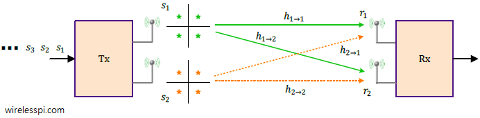
A block diagram for a multiple antenna system with $N_T$ Tx antennas and $N_R$ Rx antennas is drawn in the figure below. In this application, separate bits modulated as $s_1$, $s_2$, $\cdots$, $s_{N_T}$, are simultaneously sent through their respective Tx antennas. For example, for $N_T=2$, the first antenna sends $s_1$, $s_3$, $s_5$, $\cdots$ while the second antenna transmits $s_2$, $s_4$, $s_6$, $\cdots$.

The channel gain between $i$-th Tx antenna and $j$-th Rx antenna is denoted by $h_{(i\rightarrow j)}$. Observe on the Rx side of the above figure that the cumulative signal at each antenna is a summation of signals arriving from all Tx antennas.
\begin{equation}\label{equation-sp-general}
\begin{aligned}
r_j = h_{(1\rightarrow j)}\cdot s_1 + h_{(2\rightarrow j)}\cdot s_2 + \cdots + h_{(N_T\rightarrow j)}\cdot s_{N_T} + \text{noise}, \qquad & \\
& \qquad j = 1, 2, \cdots,N_R
\end{aligned}
\end{equation}

These equations can be written into a matrix form as
\begin{equation}\label{equation-r-matrix}
\mathbf{r=H\cdot s+\text{noise}}
\end{equation}

where

• $\mathbf{r}$ is a vector consisting of elements $r_j$, i.e., the signals arriving at Rx antennas
• $\mathbf{s}$ is a vector consisting of the modulation symbols $s_i$
• $\mathbf{H}$ is a matrix of channel coefficients

Since the signals from all Tx antennas arrive at each Rx antenna, the main task of the detection algorithms here is to free each modulated bit sent by one Tx antenna from the interference of the other modulated bits sent by rest of the Tx antennas.

How to accomplish that is where we go next.

Singular Value Decomposition (SVD)

---

Notice how Eq (\ref{equation-r-matrix}) is nothing but a matrix version of Eq (\ref{equation-single-antenna-system}). Therefore, in a similar manner to $h$ before, the matrix $\mathbf{H}$ in Eq (\ref{equation-r-matrix}) rotates and stretches the symbol vector $\mathbf{s}$!

This rotation and stretching by the matrix $\mathbf{H}$ depends on the channel coefficients $h_{(i\rightarrow j)}$. In general, such an operation results in the input vectors spreading out in all directions.

In other words, an input set of orthogonal vectors $\mathbf{V}$ when multiplied with the channel matrix $\mathbf{H}$ produces an output set of orthogonal vectors denoted by $\mathbf{U}$, which is then stretched by different scaling factors combined in a diagonal matrix $\mathbf{\Sigma}$.

Such an operation is drawn in the figure below for two vectors for illustration purpose. Here, two vectors $v_1$ and $v_2$ that are $90^\circ$ apart are multiplied with the channel matrix which results in their rotation to form vectors $u_1$ and $u_2$ that are also $90^\circ$ apart. These $u_1$ and $u_2$ are then scaled by $\sigma_1$ and $\sigma_2$, respectively, to produce the final output. Such sets of input and output vectors exist for every $\mathbf{H}$ and this property proves very useful to our system design.

In summary, we can write the SVD expression for one vector as
\begin{equation}\label{equation-svd-1}
\mathbf{H\cdot v_i} = \sigma_j\cdot \mathbf{u_j}
\end{equation}

where $i$ and $j$, or the number of input and output vectors, can be different to each other. In 2D geometry, a circle on the left of the above figure is transformed into an ellipse. The orientation of the axes are dictated by the vectors $u_j$ and the lengths of the major and minor axes by $\sigma_j$. These values $\sigma_j$ are known as singular values. The vectors $\mathbf{v_i}$ and $\mathbf{u_j}$ in Eq (\ref{equation-svd-1}) can then be combined into matrices $\mathbf{V}$ and $\mathbf{U}$, respectively, to produce the final SVD expression.

Creating Independent Pipes

---

The question is how we can utilize this knowledge about the channel matrix $\mathbf{H}$ to design a system in which final vectors at the Rx are at $90^\circ$ or orthogonal to each other. This can be accomplished as follows with the help of the figure below.

• Imagine the wireless channel represented by the matrix $\mathbf{H}$ as a black box. We just learned that vectors in the direction of orthogonal vectors $\mathbf{v_i}$ will still be orthogonal at the output of this black box (albeit at a different orientation defined by $\mathbf{u_j}$ and scaled by $\sigma_i$).
• At the input of this black box, i.e., the Tx side, we rotate our modulation symbols $s_1$, $s_2$, $\cdots$, in the direction of orthogonal vectors $\mathbf{v_i}$. This is done by multiplying the modulation vector $\mathbf{s}$ with the matrix $\mathbf{V}$ that consists of all $\mathbf{v_i}$, as illustrated in the above figure. This is virtual beamforming at the Tx side, also known as linear precoding.
• At the output of this black box, i.e., the Rx side, we de-rotate the received vectors in the opposite direction from $\mathbf{u_j}$ so that the modulation symbols become interference-free again. This is accomplished through multiplying the Rx vector with the matrix $\mathbf{U^*}$ that consists of conjugates of all $\mathbf{u_j}$. Recall that a conjugate operation keeps the magnitude the same but inverts the phases which cancels the channel effect here. This is virtual beamforming at the Rx side, also known as linear postcoding.

In this way, each modulation symbol becomes independent of all the other modulation symbols: We have forged virtually parallel pipes in the air! No complicated signal processing is required to remove their effect from each other.

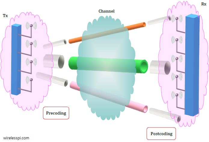
In the figure below, I have metaphorically shown this wireless channel as consisting of pipes at different orientations and thicknesses from each other that represent the vectors $90^\circ$ apart. Since the flow of fluid in any pipe does not affect the fluid in the other, this framework is now similar to the soda machine analogy.

• The pipes orientations at the left of the channel represent the directions of $\mathbf{v_i}$ towards which the Tx weights should focus the energy.
• The thickness of the pipes represents the singular values $\sigma_i$ that signify how much fluid each pipe can carry.
• The pipes orientations at the right of the channel represent the directions of $\mathbf{u_j}$ from which Rx should virtually collect the energy.

Randomly Spraying Energy

---

We earlier assumed that the number of Tx antennas $N_T$ is the same as the number of Rx antennas $N_R$ and each Tx antenna is transmitting an independent modulation symbol $s_i$. This is why we represented the singular values $\sigma_i$ with index $i$, otherwise the number of singular values depends on the minimum of $i$ and $j$.

Let us now break free from these assumptions and any number of modulation symbols can be chosen before beamforming at the Tx that determines the number of virtual pipes utilized. Notice that various linear combinations of modulations symbols are being constructed at each Rx antenna while passing through the wireless channel.

• If we do not exploit the channel knowledge at the Tx which implies an absence of weighting coefficients from $\mathbf{V}$, it is like randomly emitting the energy in various directions without really caring about the constructive summation (virtually) pointed towards the Rx.
• If we do not exploit the channel knowledge at the Rx which implies an absence of weighting coefficients from $\mathbf{U^*}$, it is like randomly collecting the energy from various directions without really caring about the constructive summation (virtually) pointed towards the orientation of pipes.

Such a scenario is depicted in the figure above. With no weighting at the Tx, this random spray of energy from the Tx does not allow an optimal injection of the fluid into the target pipes. Similarly, no weights at the Rx implies randomly collecting energy from all directions instead of the channel pipes from which the actual fluid is arriving. We have three options here.

1. Mark the fattest pipe in the channel and inject all the Tx energy into that pipe. This scheme is known as diversity precoding which maximizes the data reliability. Sometimes this scheme is also known as maximum ratio transmission. While transmitting one modulation symbol $s$, this is what we can do to focus the energy from all $N_T$ Tx antennas towards all $N_R$ Rx antennas.
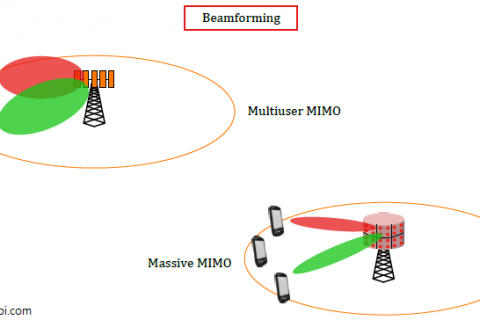
2. Direct the energy in proportion to the thickness of each pipe while transmitting independent data in each of them. This scheme is known as spatial multiplexing which maximizes the data rate. In the context of Multi-User MIMO, remember that if the terminals are sufficiently well separated then the singular vectors described above can be approximated by directional array response vectors encountered in physical beamforming.
3. Strike a balance between reliability and data rate by choosing only a few thickest pipes.

In all of these cases, linear precoding at the Tx and postcoding at the Rx needs to implemented.

Diversity Precoding

---

Diversity precoding is a special case of linear precoding in which the only target is to improve reliability and a single modulation symbol is transmitted. The precoder is one of the vectors $v_i$ we saw before in the SVD of the wireless channel. Specifically, the Tx weights are $\mathbf{v_i}$ where the index $i$ here refers to the vector corresponding to the largest singular value $\sigma_x$. As shown in the figure below, it is like pointing the whole fire hose towards the fattest pipe in the wireless channel.

In a corresponding manner, the Rx chooses the vector $\mathbf{u_j}$ as its beamforming weights where $j$ also corresponds to the index of the largest singular value $\sigma_x$. As shown in the figure above, this is like collecting all the energy from one fattest pipe only and discarding everything coming from elsewhere. This is similar to maximum ratio combination (MRC) at the Tx and MRC at the Rx in a simultaneous manner for a single symbol.

In this scenario, the equivalent model after precoding and postcoding is given by
\[
r = \sigma_x \cdot s + \text{noise}
\]

With the assumption of the modulation symbol energy normalized to 1 and noise variance given by $\sigma^2$, the SNR at the Rx can be written as
\[
SNR = \frac{\sigma_x^2}{\sigma^2}
\]

Keep in mind that in a practical implementation of this idea, it is common to take interfering signals into account as well. Then, the precoding and postcoding weights are computed according to the desired user and interfering users which maximizes the Signal to Interference plus Noise Ratio (SINR).

Closed-Loop Spatial Multiplexing

---

Diversity precoding ensures reliability but not throughput. Let us now simultaneously transmit $N$ modulation symbols where $N$ is equal to the minimum of $N_T$ and $N_R$. This choice maximizes the throughput with a sacrifice in data reliability.

• For the discussion here, channel coefficients need to be known at the Tx side which can take advantage of this information to beamform the signal in the right directions. The terminology closed-loop implies that the base station sends reference signals to the mobile terminals which then feed the channel state information back to the base station, thus ‘closing’ the loop.
• This closed-loop procedure implies a Frequency-Division Duplex (FDD) system where the Tx and the Rx occupy different frequency bands for communication. Such feedback is not required in Time Division Duplex (TDD) systems in which the Tx and Rx utilize the same frequency band but different time slots. There, the base station can estimate the channel coefficients matrix due to the principle of reciprocity: the channel at the uplink is the same as the channel in the downlink.

Recalling the idea behind the SVD of the channel matrix in Eq (\ref{equation-h-svd}), the modulation symbols are now precoded with the matrix $\mathbf{V}$ at the Tx while the received signal samples in space are postcoded with the matrix $\mathbf{U^*}$. Both of these matrices come from the SVD of the channel matrix. A symbolic representation of such a setup is drawn in the figure below where the Tx injects its energy into specific virtual pipes while the Rx collects energy from specific virtual orientations. This then becomes practically similar to point-to-point links from each Tx entity to each Rx entity.

Choosing the precoding and postcoding weights according to the channel matrix SVD is like simultaneously implementing maximum ratio transmission at the Tx and maximum ratio combining at the Rx for all modulation symbols. In these techniques, we either send the signal from Tx antennas or collect the signal energy at Rx antennas in an optimal manner that depends on the channel coefficients. Here, we are meeting at a middle ground: we focus the Tx energy in some particular directions (vectors $\mathbf{v_i}$) and gather the Rx energy from some specific directions (vectors $\mathbf{u_j}$).

Three comments are in order now.

• Creation of independent spatial pipes demands channel knowledge at both the Tx and the Rx. With channel information absent at the Tx, we talk about the open-loop mode in which no feedback is received from the Rx indicating the channel condition.
• The number of independent pipes is not the same as the number of Tx or Rx antennas. The actual number of pipes depends on something known as channel rank, i.e., the number of independent columns in the channel matrix or physically speaking the number of angular bins that can support uncorrelated entries. To emphasize this point, I have shown 4 Tx antennas, 5 Rx antennas and 3 pipes in the figure. For a rich multipath channel with signal energy arriving from all angles, this number is equal to the minimum of the Tx and Rx antennas.
• The orientations of channel pipes on the Tx side and Rx side as well as their thicknesses are different for each channel and depend on that instantaneous realization of the channel.

Finally, you might also enjoy the article on artificial intelligence.