Additive White Gaussian Noise (AWGN)

The performance of a digital communication system is quantified by the probability of bit detection errors in the presence of thermal noise. In the context of wireless communications, the main source of thermal noise is addition of random signals arising from the vibration of atoms in the receiver electronics.

You can also watch the video below.

The term additive white Gaussian noise (AWGN) originates due to the following reasons:

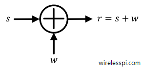
• [Additive] The noise is additive, i.e., the received signal is equal to the transmitted signal plus noise. This gives the most widely used equality in communication systems.
  \begin{equation}\label{eqIntroductionAWGNadditive}
  r(t) = s(t) + w(t)
  \end{equation}
  which is shown in the figure below. Moreover, this noise is statistically independent of the signal. Remember that the above equation is highly simplified due to neglecting every single imperfection a Tx signal encounters, except the noise itself.
  
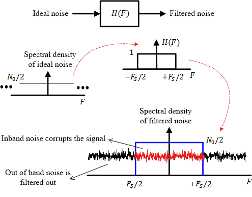
• [White] Just like the white colour which is composed of all frequencies in the visible spectrum, white noise refers to the idea that it has uniform power across the whole frequency band. As a consequence, the Power Spectral Density (PSD) of white noise is constant for all frequencies ranging from $-\infty$ to $+\infty$, as shown in Figure below.

  

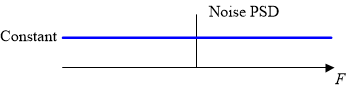
  Nyquist investigated the properties of thermal noise and showed that its power spectral density is equal to $k \times T$, where $k$ is a constant and $T$ is the temperature in Kelvin. As a consequence, the noise power is directly proportional to the equivalent temperature at the receiver frontend and hence the name thermal noise. Historically, this constant value indicated in Figure above is denoted as $N_0/2$ Watts/Hz.

  When we view the constant spectral density (we do not discuss random sequences here, so this discussion is just for a general understanding) as a rectangular sequence, its iDFT must be a unit impulse. Furthermore, we saw that the iDFT of the spectral density is the auto-correlation function of the signal. Combining these two facts, an implication of a constant spectral density is that the auto-correlation of the noise in time domain is a unit impulse, i.e., it is zero for all non-zero time shifts. This is drawn in the figure below.
  

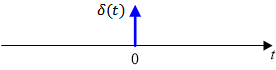
  In words, each noise sample in a sequence is uncorrelated with every other noise sample in the same sequence. Therefore, mean value of a white noise is zero.

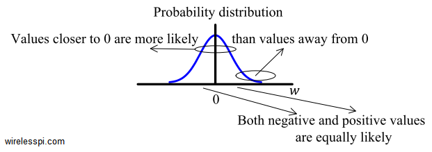
• [Gaussian] The probability distribution of the noise samples is Gaussian with a zero mean, i.e., in time domain, the samples can acquire both positive and negative values and in addition, the values close to zero have a higher chance of occurrence while the values far away from zero are less likely to appear. This is shown in the figure below. As a result, the time domain average of a large number of noise samples is equal to zero.

  

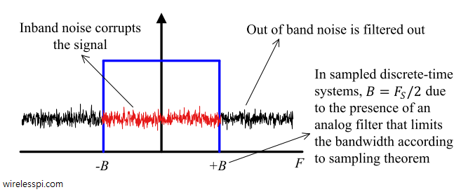
In reality, the ideal flat spectrum from $-\infty$ to $+\infty$ is true for frequencies of interest in wireless communications (a few kHz to hundreds of GHz) but not for higher frequencies. Nevertheless, every wireless communication system involves filtering that removes most of the noise energy outside the spectral band occupied by our desired signal. Consequently, after filtering, it is not possible to distinguish whether the spectrum was ideally flat or partially flat outside the band of interest. To help in mathematical analysis of the underlying waveforms resulting in closed-form expressions — a holy grail of communication theory — it can be assumed to be flat before filtering.

For a discrete signal with sampling rate $F_S$, the sampling theorem dictates that the bandwidth of a signal is constrained by a lowpass filter within the range $\pm F_S/2$ to avoid aliasing. For the purpose of calculations, this filter is an ideal lowpass filter with
\begin{equation*}
H(F) =
\begin{cases}
1 & -F_S/2 < F < +F_S/2 \\ 0 & \text{elsewhere} \end{cases} \end{equation*} The resulting in-band power is shown in red in the figure below, while the rest is filtered out.

As with all densities, the value $N_0$ is the amount of noise power $P_w$ per unit bandwidth $B$.
\begin{equation}\label{eqIntroductionNoisePower1}
N_0 = \frac{P_w}{B}
\end{equation}
For the case of real sampling, we can plug $B=F_S/2$ in the above equation and the noise power in a sampled bandlimited system is given as

Thus, the noise power is directly proportional to the system bandwidth at the sampling stage.

An AWGN channel is the most basic model of a communication system. Some examples of systems operating largely in AWGN conditions are space communications with highly directional antennas and some point-to-point microwave links. While several imperfections are still present (e.g., carrier and timing offsets), the underlying signal structure stays intact leading to a simpler Rx design because no channel equalizer needs to be incorporated.