A carrier phase offset rotates the Rx constellation causing decision errors even in a perfectly noiseless environment. One of the techniques used to overcome this problem is to insert a known sequence at the start of the transmission known as a preamble. Then, the Rx can utilize these known symbols in the arriving signal to estimate the carrier phase and de-rotate the constellation.
However, inserting a known sequence within the message decreases the spectral efficiency of the system. To avoid this cost, a phase estimator (as well as estimators for other distortions) can be derived in a non-data-aided fashion. One option is to use decision-directed strategies in which the outputs of the decision device are used as a replacement of the known data. However, this strategy cannot be utilized for initial phase acquisition at the start of the transmission because the phase offset can be large causing errors in data decisions as well as synchronization estimate.
Let us start with the M-th power estimator taking an example of a QPSK constellation. Later, it can be generalized to an MPSK modulation scheme. Recall from the discussion on complex numbers that in an $IQ$-plane, raising a complex number to a certain power raises the magnitude to that power while multiplies the phase with that number. For a complex number $V$ in polar form and its 4-th power,
\begin{aligned}
|V^4| &= |V|^4 \\
\measuredangle ~V^4 &= 4\cdot \measuredangle ~V
\end{aligned}
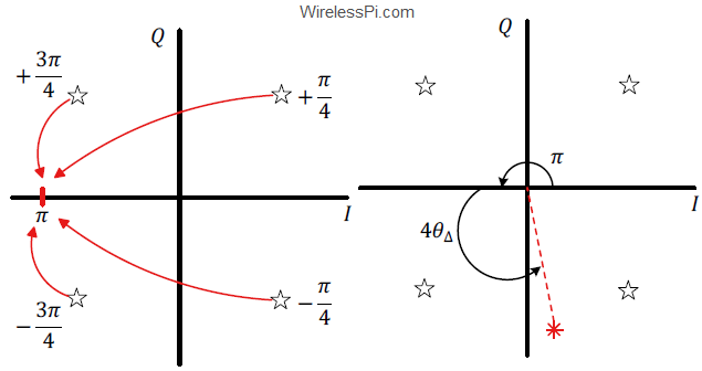
The phases of the four points on a regular QPSK constellation are given by $\pm \pi/4$ and $\pm 3\pi/4$. Since
\begin{equation*}
+\pi = -\pi = +3\pi = -3\pi,
\end{equation*}
multiplying these phases with $4$ maps them all to the same location.
\begin{equation*}
4\cdot \Big\{ \pm \frac{\pi}{4}, \pm \frac{3\pi}{4}\Big\} = \pi
\end{equation*}
This phase multiplication, for QPSK symbols $a[m]$, can be written as
\begin{equation*}
4\cdot \measuredangle ~a[m] = \pi
\end{equation*}
regardless of the value each $a[m]$ has. The underlying intuition behind this is the $2\pi/4$ rotational symmetry of QPSK constellation: rotating the constellation by an angle of $2\pi/4$ generates the same constellation. This can be implemented by raising $a[m]$ to the 4-th power and is drawn on the left side of the figure below. We can see that the 4-th power operation has removed the modulation from all data points without any data knowledge at the Rx.

With this background, let us consider the case where the QPSK symbols at the Rx contain a phase offset $\theta_\Delta$ as well. We use the following notations.
- The data symbols are denoted by $a[m]$ whose inphase and quadrature parts are $a_I[m]$ and $a_Q[m]$ respectively).
- The matched filter output at the Rx, downsampled to 1 sample/symbol, is denoted by $z(mT_M)$ where $m$ is the symbol index and $T_M$ is the symbol duration.
Now recall from the article regarding the effect of carrier phase offset that the magnitude and phase of the matched filter output at symbol interval $m$ can be written as
\begin{equation*}
\begin{aligned}
|z(mT_M)| &= \sqrt{a_I^2[m] + a_Q^2[m]} \\
\measuredangle ~z(mT_M) &= \measuredangle ~a[m] + \theta_\Delta
\end{aligned}
\end{equation*}
where a mismatch of $\theta_\Delta$ between incoming carrier and Rx oscillator is seen to leave the magnitude of the data symbols $a[m]$ unchanged and rotate their phases by an angle $\theta_\Delta$. Clearly, raising each output to the 4-th power yields
\begin{equation*}
\begin{aligned}
|z^4(mT_M)| &= \Big(a_I^2[m] + a_Q^2[m]\Big)^2 \\
\measuredangle ~z^4(mT_M) &= 4\cdot \measuredangle~ a[m] + 4\theta_\Delta = \pi + 4\theta_\Delta
\end{aligned}
\end{equation*}
This is illustrated on the right side of the figure above. In the above equation, the summation of matched filtered outputs can be employed to average the noise and a non-data-aided phase estimator can be derived as
\hat \theta_\Delta = \frac{1}{4}\cdot \measuredangle~\left\{\sum _{m=0} ^{N_d-1} z^4(mT_M) \right\} – \frac{\pi}{4}
\end{equation}
where $N_d$ is the sequence length in symbols.
For another version of QPSK constellation, the symbols start from an angle $0$ instead of $\pi/4$. Hence, its phase values are
\begin{equation*}
0, +\frac{\pi}{2}, \pi, -\frac{\pi}{2}
\end{equation*}
which after multiplication by $4$ all map to the an angle $0$. In this case, the factor $\pi/4$ is not required.
\begin{equation}\label{eqPhaseSyncMPower42}
\hat \theta_\Delta = \frac{1}{4}\cdot \measuredangle~\left\{\sum _{m=0} ^{N_d-1} z^4(mT_M) \right\}
\end{equation}
This is the most common form of 4-th power estimator encountered in the synchronization literature.
The above estimator works due to $2\pi/4$ rotational symmetry of the QPSK constellation. For a general $M$-PSK constellation with a rotational symmetry of $2\pi/M$ and the starting phase of $0$, the M-th power phase estimator can be written as
\begin{equation*}
\hat \theta_\Delta = \frac{1}{M}\cdot \measuredangle~\left\{\sum _{m=0} ^{N_d-1} z^M(mT_M) \right\}
\end{equation*}
A block diagram of this scheme is drawn in the figure below. Notice the absence of any training data, presence of an M-th power operation and a $1/M$ scaling factor.

Now let us turn our attention to what happens in the presence of noise. For the simple case of raising the matched filter output to the 4-th power and using the identity $(A+B)^4 = A^4+4A^3B + 6A^2B^2 + 4AB^3+B^4$,
\begin{align*}
(\text{signal}+\text{noise})^4 &= \text{signal}^4+4\times \text{signal}^3\times \text{noise} + 6\cdot \text{signal}^2\times \text{noise}^2 + \\
&\hspace{2in} 4\cdot \text{signal} \times \text{noise}^3+ \text{noise}^4
\end{align*}
Here, we have four terms that involve noise. A consequence of the power operation is now clear: significant noise enhancement in the estimation block. In general, a larger $M$ yields a larger phase jitter at the NCO output. Subsequently, the performance of non-data-aided schemes is worse than data-aided techniques. This loss in performance is the price paid for the absence of training sequence in the packet for increasing spectral efficiency.
Another non-data-aided system can be built from feedback techniques, like a Phase Locked Loop (PLL). Assume that a PLL is employed for synchronizing the Rx oscillator phase to the phase of the Tx signal. In this situation as well, the Rx PLL can be driven through the actual Tx signal itself and without any pilot tone if the phase shifts at symbol intervals arising from modulating data can be removed.
Most PLLs operate either in a data-aided manner or through the decisions fed back from the detector. When no such help is available, our initial idea to modify a simple PLL in non-data-aided mode is the following.
- At each symbol time $mT_M$, raise the matched filter output to M-th power and employ it as a phase error detector.
- At next symbol time $(m+1)T_M$, de-rotate the matched filtered output through the NCO output.
- At this symbol time $(m+1)T_M$, use this de-rotated matched filtered signal as the phase error detector input.
Subsequently transform the feedforward M-th power estimator $\hat \theta_\Delta$ explained above into a feedback phase error detector output $e_D[m]$ by
- removing the summation, and
- replacing the matched filter output $z(mT_M)$ by de-rotated matched filter output
as
\begin{equation}\label{eqPhaseSyncMPowerPED}
e_D[m] = \frac{1}{M}\cdot \measuredangle~z^M(mT_M)
\end{equation}
As opposed to wiping off the carrier phase offset once and for all as done in feedforward M-th power estimator, this kind of implementation is essentially a strategy to converge towards the final solution in small incremental steps. The rest of the principles remain the same as in an ordinary PLL and data-aided/decision-directed approaches explained above. On the downside, the phase detection range of the M-th power PED is reduced to $[-\pi/M, +\pi/M)$ due to the phase ambiguity. This is because raising a carrier to the M-th power generates a control signal that represents $M$ times the actual phase difference.
A well known phase synchronization technique for BPSK modulation, known as the squaring synchronizer, is a special case of M-th power synchronizer with $M=2$.
\begin{equation*}
e_D[m] = \frac{1}{2}\cdot \measuredangle~\overset{\curvearrowright}z^2(mT_M)
\end{equation*}
The squaring operation removes the modulation and doubles the frequency which is locked through a standard PLL. The output of the PLL is divided by $2$ to provide the carrier at the actual frequency which is then used to synchronously demodulate the Rx signal. A block diagram of a squaring synchronizer directly operating on the Rx BPSK signal is drawn in the figure below. The squaring synchronizer has been extensively used for locking the carrier in conventional amplitude modulated systems of the past years.