Effect of Sampling Clock Offset on a Single-Carrier Waveform

We have discussed before the distortion caused by a symbol timing offset on the communication waveform. We have also derived a maximum likelihood estimate of the clock phase offset. In this article, we describe the impact of a sampling clock offset in a single-carrier waveform, also commonly known as a clock frequency offset or timing drift. A clock frequency offset is defined as the rate mismatch between the Tx and Rx clocks.

Just like a carrier phase and frequency offset, the clock used to sample the incoming continuous-time signal at a rate $T_S=1/F_S$ contains a phase and frequency offset as compared to the Tx clock as well. However, there is a difference between the treatment of timing phase and frequency offsets as compared to the carrier phase and frequency offsets as follows.

• The accuracy of the local oscillators in communication receivers is defined in terms of ppm (parts per million) such as 1 ppm is 1 out of $10^6$ parts. For example, with $F_C=1.9$ GHz and $\pm 20$ ppm crystals,
  \begin{equation*}
  \pm \frac{20}{10^6} \times 1.9 \times 10^9 = \pm 38 ~\text{kHz}
  \end{equation*}

  For the purpose of typical wireless communication systems operating at several hundreds of MHz or GHz of carrier frequency $F_C$, it is one of the major sources of signal distortion. This problem gets worse at higher mmWave frequencies used for 5G cellular systems.

• On the other hand, typical symbol rates in a wireless system are typically on the order of several MHz (modern wireless systems such as 5G cellular and WiFi are breaking into GHz symbol rates now). Consider an example of a wireless system operating at a symbol rate of $5$ MHz and with $\pm 20$ ppm crystals. The maximum deviation of the timing frequency at the Tx or Rx can be
  \begin{equation*}
  \pm \frac{20}{10^6} \times 5 \times 10^6 = \pm 100 ~\text{Hz}
  \end{equation*}

  For such transmission speeds, a symbol timing frequency offset poses much less of a distortion as compared to a carrier frequency offset. Nonetheless, it is necessary to compensate in most wireless systems to match the Tx symbol rate due to extra samples injected into or deleted from the symbol stream.

For a normalized sampling clock offset of $\zeta$, the Rx sample time is given by
\begin{equation*}
\tilde{T}_S = T_S(1+\zeta)
\end{equation*}

A common analogy that captures this concept is driving on a highway next to a train line. Either the car is faster or slower than the train and you can see how a small initial speed difference culminates in one vehicle completely left behind. Our bodies also function on free-running biological clocks slightly unsynchronized with the 24-hour day and night cycle. Scientists have actually verified that a complete isolation from the outside world makes our sleep and wake-up patterns drift away.

The sampling clock offset $\zeta$ can be greater or lesser than the ideal value of $0$ which determines whether the Rx clock is slower or faster than the Tx clock as described below.

$\zeta>0$

---

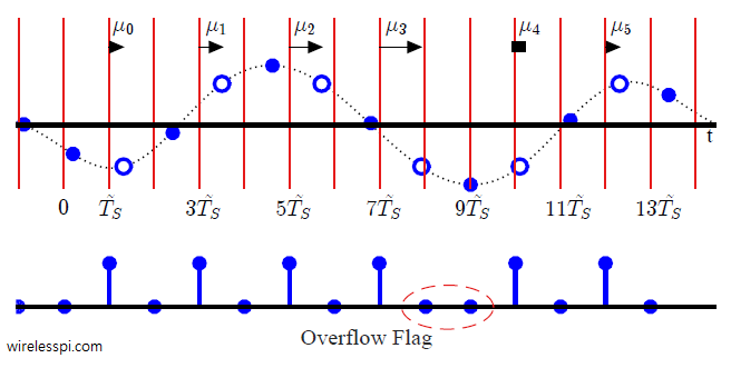
This implies that $\tilde{T}_S-T_S>0$ or $\tilde{T}_S>T_S$, i.e., the Rx clock is slower than the Tx clock. Therefore, the Rx does not collect exactly $L$ samples in a symbol period $T_M$ as shown in the figure below for (an impractically large) $\zeta=1.1$. Ideally, the Rx should sample the waveform (shown by red vertical lines) at the locations of Tx samples shown as circles.

In the above figure, assume an ideal scenario where the fractional interval $\mu_m$ is the same as the actual timing offset and let us focus on the fractional interval $\mu_m$ (represented by the time difference between a red dashed line and white circle) for $L=2$. Observe that although the effect of $\zeta>0$ is initially small, the error accumulates with time and $\mu_0$ at $\tilde{T}_S$ is larger than $\mu_1$ at $3\tilde{T}_S$. It keeps decreasing until it reaches zero around $9\tilde{T}_S$ and wraps around zero at $10\tilde{T}_S$! The main point here is that the overflow that occurs every $L=2$ samples now occurs at the very next sample — at both $9\tilde{T}_S$ and $10\tilde{T}_S$ — implying that the loop has missed a sample due to its slow rate. The wrap around of the fractional interval from $0$ to $1$ is an indication that a missing sample needs to be inserted in the timing error detector registers, one indication of which is that the overflow flag is high at two consecutive samples as shown in the figure.

$\zeta<0$

---

This implies that $\tilde{T}_S-T_S<0$ or $\tilde{T}_S < T_S$, i.e., the Rx clock is faster than the Tx clock. In the figure below, again assume an ideal scenario where the fractional interval $\mu_m$ is the same as the actual timing offset. Observe that the error accumulates with time and $\mu_1$ at $3\tilde{T}_S$ is larger than $\mu_0$ at $\tilde{T}_S$. It keeps increasing until it reaches close to one around $7\tilde{T}_S$ and then wraps around one at $10\tilde{T}_S$! The main point here is that the overflow that occurs every two samples now occurs at a gap of $3$ samples, implying that the Rx has inserted an extra sample due to its fast rate. The wrap around of the fractional interval from $1$ to $0$ is an indication that an extra sample needs to be deleted from the TED registers, one indication of which is that the overflow flag is low at two consecutive samples as shown in the figure.

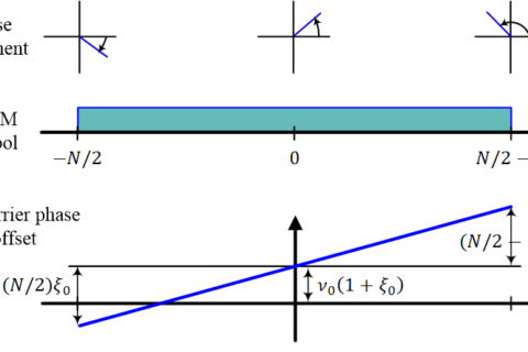
The effect of a sampling clock offset on an OFDM waveform is a little different, as it is proportional to the subcarrier index.