Rabbits, Foxes and IQ Signals

If we pay attention, each term in a mathematical equation carries a meaning that resonates with common sense. Today I will explain where Lotka-Volterra equations come from. These equations describe the dynamics of a biological interaction in which a predator (e.g., foxes) and a prey species (e.g., rabbits) engage with each other in a continuous struggle for survival.

We will see that the math expressions just line up to describe the phenomenon almost as in words. Moreover, they have a little connection to IQ signals, the fundamental concept in digital signal processing, that will also be presented in the article.

Let us start with the expressions for the predator-prey model.

A Tale of Survival

Our target is to track the populations of both the predator and prey and how they change over time. We assume that the prey has unlimited resources of food while the predator only relies on the prey for its survival.

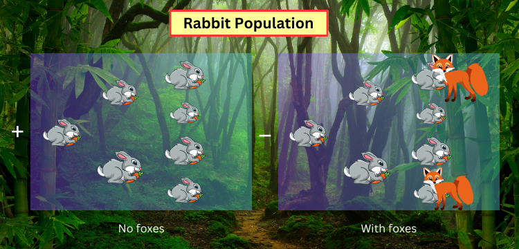
In these conditions, we expect that the predator population grows when there is a plentiful supply of prey. However, this rise in predators leads to a decline in the number of prey. When prey becomes scarce, the number of predators decreases. This reduction in predators allows the prey population to rise again, perpetuating the cycle.

Since both predator and prey start with the letter $p$ and general terms like $x$ and $y$ do not indicate towards them, let us denote the population (or population density) of the prey by $r$ (the rabbit) and that of the predator by $x$ (the fox). The dynamic system is then governed by the following equations.
\[
\begin{aligned}
\frac{dr}{dt} &= \alpha r ~- \beta rx \\\\
\frac{dx}{dt} &= -\gamma x + \delta rx
\end{aligned}
\]

Although they appear complicated at first glance, dissecting these terms one by one unveils their inherent logic, which is what we do next.

Rabbit Population $r$

In the given setup, there are two ways in which the rabbit population $r$ can change.

• A positive growth rate due to reproduction is determined by a constant $\alpha$. This gives rise to the term $\alpha r$ that points towards an exponential growth. Why? Because an exponential function is a derivative of itself.
  \[
  \frac{d\left(e^t\right)}{dt} = e^t
  \]

  In real life, reproduction is indeed exponential (if the resources are unlimited) where two become four, four become eight and so on.

  

• A negative growth rate occurs due to predation governed by a constant $\beta$ that captures the effect of the foxes on the rabbits’ death rate. This yields the other term $-\beta rx$. The multiplication comes from the fact that the whole rabbit population is a possible target for each individual fox. The rate of preying depends on how often they meet (this will be zero if either $r$ or $x$ is zero).

Combining the above two provides us with the final equation.
\begin{equation}\label{equation-lotka-volterra-prey}
\frac{dr}{dt} = \alpha r~ – \beta rx
\end{equation}

In words, the above equation tells us that the fluctuation in the rabbit population is calculated by its positive growth rate, minus the rate at which it is preyed upon.

We now move towards the predator, the foxes.

Fox Population $x$

Again, there are two ways in which the fox population $x$ can change.

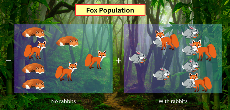
• A negative growth rate due to natural death determined by a constant $\gamma$. This gives rise to the term $-\gamma x$. Similar to the rabbits, this is also an exponential decay because starvation affects every fox regardless of its age and the prey is the only food source.

  

• A positive growth rate due to predation governed by a constant $\delta$ that captures the effect of the hunting activity on the predator. This yields the other term $+\delta rx$ where we saw above the reason behind the multiplication. However, the factor $\gamma$ is not the same as $\beta$ because predation has a different impact on foxes’ growth rate as compared to the rabbits’ death rate.

Combining the above two provides us with the final equation.
\begin{equation}\label{equation-lotka-volterra-predator}
\frac{dx}{dt} = -\gamma x + \delta rx
\end{equation}

In words, the above equation tells us that the predator population changes according to the pace at which it consumes prey less its inherent death rate.

We can now write the whole system model from Eq (\ref{equation-lotka-volterra-prey}) and Eq (\ref{equation-lotka-volterra-predator}) as

This is how an apparently complicated system becomes simpler when the logic behind each term is explained.

The Solution

The above dynamic system does not have a simple solution. So we will not derive it here and instead rely on simulations. Keep in mind that the discrete-time version of this system can also be tracked using an extended version of the Kalman filter.

The cycle of fox-rabbit population dynamics is shown in the figure below for a particular set of $\alpha$, $\beta$, $\gamma$ and $\delta$. These populations interact with one another in accordance with Eq (\ref{equation-lotka-volterra}).

• It is evident that a population of rabbits will grow exponentially with an unlimited food supply and no foxes.
• However, with an abundance of prey around, the population of foxes increases.
• This rise in their population brings the rabbit population down.
• With a dwindling number of rabbits around, fox population is forced to decrease as well.

This cycle of growth and decline in populations is metaphorically the heartbeat of life in the cosmic theatre.

The most important point to remember is the following.

Let us redraw the above figure with the population of rabbits on x-axis while that of the foxes on y-axis. This is known as a phase plot which demonstrates the same relationship between the two species disregarding the time.

We now move from survival towards competition.

A Tale of Competition

The irregular shape of the phase plot in the above figure is due to the asymmetries between predator and prey. What if there were two species of animals who hunt each other, i.e., both are predator and prey at the same time?

Usually this does not happen in nature as it would be an evolutionary mistake. Preying upon a similarly sized species would cause a significant risk of injury, exhaustion or death for the predator. This is why animals seek out smaller and easier targets, even in groups. Strangely, humans took a long time to learn something that animals understand by nature. It was only after two world wars and an inconceivable destruction that powerful states finally stopped fighting each other and went back to invading weaker countries again.

But if there was such a pair of big animals (e.g., a caiman and an anaconda), how would the above plots look like? Changing the values of the parameters, we get the time plot of the two populations in the figure below. It is clear that the two populations are a close match, one species nearly wipes out the other which in turn rises to do the same and the cycle continues.

Notice how these curves are similar to a cosine and sine with a phase difference of $90^\circ$. The phase plot, i.e., a plot between populations of predators, is shown below. It is almost approaching a circle, pointing towards the symmetry in the interaction.

We now relate this plot to IQ signals.

An IQ Signal

In reality, the time axis exits in a 3rd dimension coming out of the page. To see this, let us redraw the above figure for a perfect competition on a complex plane with axes denoting real and imaginary parts, instead of Predator 1 and Predator 2. As a consequence, the plot assumes the shape of a helix (notice the circle from the front view) whose rate of rotation is given by $\omega=2\pi f$ (think of simple harmonic motion on side walls).

This is the fundamental IQ signal in DSP known as a complex sinusoid and its mathematical expression is given by
\[
e^{j2\pi ft} = \cos 2\pi ft + j \sin 2\pi ft
\]

Just like the population of the predator trailing that of the prey by $90^\circ$ before, the sine wave lags behind the cosine by $90^\circ$!

So what is an IQ signal? Just like a complex number has a real and imaginary part, a IQ signal has a real and imaginary part, i.e., it is also a complex number. The only difference is that it is evolving with time (a different complex number at each instant) which is why it is also known as a complex signal.

Conclusion

The article describes the competition between two species and how it forms a periodic behavior over time. When the two species are equally matched, this becomes quite similar to a complex number evolving in time. Such a combination of complex numbers (one at each time instant) is known as a complex or IQ signal.

If you want to learn more about IQ signals from a communications perspective, see the article IQ signals 101 – Neither complex nor complicated.