Usually a modulation of one species can only be demodulated with the radio signal processing chain of the same species. But P25 has a very interesting and unusual concept of demodulating a signal from one modulation species using the receiver of another species.
APCO Project 25, commonly known as P25, is a suite of digital radio standards designed for public safety and first responder communications across North America which is similar to European Terrestrial Trunked Radio (TETRA). The main purpose of its development was to ensure seamless interoperability among federal, state and local agencies. Hence, it enables radios from different manufacturers to communicate on the same network.
The standard is split into two phases: Phase 1 and Phase 2. Our focus today is on Phase 1. There are two modulation schemes defined in the standard, C4FM (Compatible 4-Level Frequency Modulation) and CQPSK (Compatible Quadrature Phase Shift Keying), both of which operate at a rate of $4800$ symbols/second and convey 2 bits of information per symbol. The symbol time, therefore, is given by
\[
T_M = \frac{1}{4800} \approx 208 ~\mu \text{s}
\]
P25 radio systems are designed in a way that a CQPSK signal can be demodulated with a receiver designed for C4FM signals. To see how a QPSK type linearly modulated signal goes through each block of a 4-FSK type receiver and still generate the correct output, let us start with the description of a C4FM modulator.
C4FM Modulator
A block diagram of the C4FM modulator is drawn in the figure below.

Each block of this modulator is now discussed in detail.
4-PAM Lookup Table
The processing on Tx side starts with a serial-to-parallel converter that picks up two bits at one time and inputs them into a lookup table (LUT). This lookup table outputs the symbols corresponding to the bit pair, similar to a Pulse Amplitude Modulation (PAM) system.
The mapping from the bit pair to the symbol might look strange, as it is not following a natural sequence as in digital logic. This is due to the Grey coding in which the adjacent symbols only differ in one bit. This helps reduce the bit error rate when the symbol errors inevitably occur.
The output of this lookup table is a sequence of symbol-spaced impulses $a[m]$ with amplitudes $\pm 1$ or $\pm 3$. This sequence is upsampled by a factor of $L$ samples/symbol to make room for the pulse shape coming next.
Raised Cosine Filter $H(f)$
The upsampled sequence of symbols is input to a Raised Cosine filter, the details of which you can see in pulse shaping filter. The expression for a Raised Cosine in frequency domain is given by
\[
H(f) = \left\{ \begin{array}{l}
1 \hspace{3.3in} 0 \le |f| \le \frac{1-\alpha}{2T_M} \\ \\
\frac{1}{2}\left[1 + \cos \left\{2\pi \frac{T_M}{2\alpha} \left( |f| – \frac{1-\alpha}{2T_M}\right)\right\} \right]
\hspace{0.5in} \frac{1-\alpha}{2T_M} \le |f| \le \frac{1+\alpha}{2T_M} \\ \\
0 \hspace{3.3in} |f| \ge \frac{1+\alpha}{2T_M}
\end{array} \right.
\]
where $T_M$ is the symbol time and $\alpha$ is the excess bandwidth or rolloff factor.
The P25 Phase 1 standard defines $\alpha=0.2$. Plugging this value along with $T_M =1/4800$ implies that the frequency domain expression becomes
\[
H(f) = \left\{ \begin{array}{l}
1 \hspace{3.2in} 0 \le |f| \le 1920~\text{Hz} \\ \\
\frac{1}{2}\left[1 + \cos \left\{\frac{2\pi}{1920}\left(|f|-1920\right)\right\}\right] \hspace{0.5in} \text{for }1920~\text{Hz} \le |f| \le 2880~\text{Hz} \\ \\
0 \hspace{3.2in} \text{for } |f| \ge 2880~\text{Hz}
\end{array} \right.
\]
A frequency domain diagram of the resulting Raised Cosine filter for $\alpha=0.2$ is drawn in the figure below.

The impulse response $h[n]$ can be derived through an inverse Fourier Transform. The resultant waveform in time domain is equivalent to product of a sinc signal with an even signal of time.
\[
h [n] = \frac{1}{L}\cdot \frac{\sin(\pi n/L)}{\pi n/L} \cdot \frac{\cos (\pi \alpha n/L)}{1-\left(2 \alpha n/L\right)^2}
\]
The above equation becomes indeterminate for $n=0$ and $n = \pm L/(2\alpha)$. It can be shown through L’Hopital’s rule that
\begin{align*}
h[0] &= 1 \\ \\
h[\pm \frac{L}{2\alpha}] &= \frac{\alpha}{2} \sin \frac{\pi}{2\alpha}
\end{align*}
This impulse response is drawn in the figure below for $\alpha=0.2$. Note the zero crossings of the waveforms at integer multiples of $T_M$.

A common convention in communication systems is to use a Root Raised Cosine at the Tx and another Root Raised Cosine at the Rx. The reason for utilizing the whole Raised Cosine spectrum at the Tx here is to control the spectrum more efficiently within the prescribed $12.5$ kHz bandwidth.
Shaping Filter $P(f)$
This terminology is a little unusual since the term shaping filter is generally reserved for pulse shaping filters like the Raised Cosine above. The shaping filter here is defined as
\[
P(f) = \frac{\pi f/4800}{\sin \left(\pi f/4800\right)} \qquad |f| \le 2880~ \text{Hz}
\]
From DFT of a rectangular pulse, we know that this is an inverse sinc filter that pre-emphasizes high frequencies of the signal. There is a corresponding sinc filter on the Rx side in the form of a moving average (because the Fourier Transform of a rectangular impulse response like a moving average is a sinc function in frequency), commonly known as an integrate-and-dump filter. The cascade of both of these filters approaches a flat response within the signal bandwidth. This is plotted in the figure below.

The baseband signal is now a 4-PAM upsampled symbol stream filtered by
\[
G(f) = H(f)\cdot P(f), \qquad \text{or}\qquad g[n] = h[n]*p[n]
\]
This enables us to write the mathematical expression for the input to the FM modulator as
\begin{equation}\label{equation-4-pam}
x(t) = \sum _{m} a[m] g(t-mT_M)
\end{equation}
sampled at $t=nT_s$, where $a[m]$ are symbol values $\pm 1$ or $\pm 3$ and $T_M$ is the symbol duration. Next, we turn our attention towards FM modulator.
FM Modulator
In a discrete-time implementation for FM with a sample rate $F_s=1/T_s$ and input $x[n]$, we integrate the phase after including the frequency deviation $k_f$.
$$\begin{equation}
\begin{aligned}
\theta(nT_s) &= 2\pi k_f \int_{0}^{nT_s} x(\tau) d\tau \\
&= 2\pi k_f \int_{0}^{(n-1)T_s} x(\tau) d\tau + 2\pi k_f \int_{(n-1)T_s}^{nT_s} x(\tau) d\tau \\ \\
&=\theta[(n-1)T_s] + 2\pi k_f T_s x(nT_s)
\end{aligned}
\end{equation}\label{equation-fm-phase-baseband}$$
where $k_f$ is the frequency deviation equal to $600$ Hz here and the continuous-time integral can be replaced with the forward difference or backward difference version (with $x[(n-1)T_s]$) of a discrete-time integrator.
A block diagram of a discrete-time FM modulator is now drawn in the figure below where $D$ denotes a unit time delay commonly written as $z^{-1}$. The Look-Up Table (LUT) stores the values of cosine and sine functions. The complete setup forms a Numerically Controlled Oscillator (NCO) for FM signal generation. The NCO combined with a Digital to Analog Converter (DAC) turns into a Direct Digital Synthesizer (DDS) implementation.
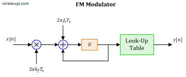
As a result, the output $y[n]$ is a complex exponential at a frequency $f_c$ that is written as
\begin{equation}\label{equation-discrete-fm}
y[n] = A_c e^{j\left[2\pi f_c nT_s ~+~ \theta(nT_s)\right]}
\end{equation}
From the above expression, it is easy to see the relationship between information bit pairs and total frequency deviation, as shown in the table below.
| Information Bits | Symbol | C4FM Deviation |
|---|---|---|
| 01 | +3 | +1.80 kHz |
| 00 | +1 | +0.60 kHz |
| 10 | -1 | -0.60 kHz |
| 11 | -3 | -1.80 kHz |
C4FM Demodulator
To focus on the signal processing operations, let us remove the carrier term by multiplying $y[n]$ in Eq (\ref{equation-discrete-fm}) with $e^{-j2\pi f_c nT_s}$ and assume that $A_c$ is equal to 1 for simplicity.
\[
z[n] = y[n]e^{-j2\pi f_c nT_s} = e^{j\theta(nT_s)}
\]
What happens when the above signal is multiplied with a delayed and conjugated version of itself?
\[
v[n] = z[n]\cdot z^*[n-1]
\]
Since a conjugate operation reverses the phase sign, we have
\[
v[n] = e^{j\theta(nT_s)}\cdot e^{-j\theta[(n-1)T_s]} = e^{j\left\{\theta(nT_s) – \theta[(n-1)T_s]\right\}}
\]
We deduce that conjugate multiplication computes the difference between phases. Using Eq (\ref{equation-fm-phase-baseband}), what remains is the 4-PAM waveform, $x(nT_s)$, in the exponential.
\begin{equation}\label{equation-fm-demodulation}
v[n] = e^{j 2\pi k_f T_s x(nT_s)}
\end{equation}
Apparently, this is a delayed conjugate product operation used in many signal processing applications. Behind the scene, this is an implementation of a discrete-time first-difference differentiator.

Finally, taking the angle through atan2( ) operation, we get
\[
\measuredangle v[n] = 2\pi k_f T_s \cdot x(nT_s)
\]
which is our desired message signal scaled by $2\pi k_f T_s$.
\[
x(nT_s) = \frac{1}{2\pi k_f T_s}\measuredangle v[n]
\]
This recovers the original 4-PAM waveform from Eq (\ref{equation-4-pam}) to be demodulated by a conventional linear demodulator.
CQPSK Modulator
The CQPSK modulator is a typical Quadrature Amplitude Modulation (QAM) Tx with separate $I$ and $Q$ rails. The block diagram is drawn in the figure below.

Here, a serial-to-parallel (S/P) converter collects $2$ bits every $T_M = 1/4800$ seconds that are used as an address to access two Look-Up Tables (LUT), the outputs of which are selected according to a $\pi/4$ DQPSK modulation. Here the absolute phase state $\theta[m]$ is recursively updated using the previous phase state $\theta[m-1]$ and the current information-bearing phase shift $\Delta \theta[m]$.
\theta[m] = \theta[m-1] + \Delta \theta[m] \qquad (\text{mod}~2\pi)
\end{equation}
The phase change $\Delta \theta[m]$ is computed as a multiple of $45^\circ$ as shown in the table below.
| Information Bits | Symbol | CQPSK Phase Change $\Delta \theta[m]$ |
|---|---|---|
| 01 | +3 | +135 degrees |
| 00 | +1 | +45 degrees |
| 10 | -1 | -45 degrees |
| 11 | -3 | -135 degrees |
From this table, the bit pair 01 requires a +135° ($3\pi/4$ radians) phase shift over the symbol time $T_M$ (instead of an instant jump due to filtering). Since symbol rate $1/T_M$ is 4800 Hz, we get the frequency equivalent of this phase change as
\[
\frac{3\pi}{4}:2\pi :: x:4800
\]
which implies that
\[
\frac{3\pi/4}{2\pi} = \frac{x}{4800}, \qquad \text{or} \qquad x = 1800~\text{Hz}
\]
This 1800 Hz is exactly the +3 frequency deviation in C4FM table before.
While the actual modulation conveys 2 bits per symbol, there are 8 points on the constellation diagram due to its differential nature. This is plotted in the figure below.

These 8 distinct phase positions, distributed uniformly around a circle, represent the interleaving of two separate 4-point QPSK constellations over time. The signal only ever transitions from a blue dot to a red dot, or a red dot to a blue dot. It never stays on the same set or jumps between points of the same color. This implies that both $I$ and $Q$ lookup tables consist of $5$ values ($0$, $\pm 1$ and $\pm 0.7071$), as shown in the table below.
To decode how the entries of this table are filled, consider the following. In phase state 0 (i.e., $I=1$, $Q=0$), the arrival of information bits 00 changes the phase by $+45^\circ$ according to the above table. This implies that we reach an angle of $45^\circ$ on the unit circle, or $I=0.7071$, $Q=0.7071$, which is phase state 1. The rest of the table can be decoded in the same way.
| $\theta[m-1]$ State | Information Bits |
$\theta[m]$ State | I Level | Q Level |
|---|---|---|---|---|
| 0 | 00 | 1 | +0.7071 | +0.7071 |
| 0 | 01 | 3 | -0.7071 | +0.7071 |
| 0 | 11 | 5 | -0.7071 | -0.7071 |
| 0 | 10 | 7 | +0.7071 | -0.7071 |
| 1 | 00 | 2 | +0.0 | +1.0 |
| 1 | 01 | 4 | -1.0 | +0.0 |
| 1 | 11 | 6 | +0.0 | -1.0 |
| 1 | 10 | 0 | +1.0 | +0.0 |
| 2 | 00 | 3 | -0.7071 | +0.7071 |
| 2 | 01 | 5 | -0.7071 | -0.7071 |
| 2 | 11 | 7 | +0.7071 | -0.7071 |
| 2 | 10 | 1 | +0.7071 | +0.7071 |
| 3 | 00 | 4 | -1.0 | +0.0 |
| 3 | 01 | 6 | +0.0 | -1.0 |
| 3 | 11 | 0 | +1.0 | +0.0 |
| 3 | 10 | 2 | +0.0 | +1.0 |
| 4 | 00 | 5 | -0.7071 | -0.7071 |
| 4 | 01 | 7 | +0.7071 | -0.7071 |
| 4 | 11 | 1 | +0.7071 | +0.7071 |
| 4 | 10 | 3 | -0.7071 | +0.7071 |
| 5 | 00 | 6 | +0.0 | -1.0 |
| 5 | 01 | 0 | +1.0 | +0.0 |
| 5 | 11 | 2 | +0.0 | +1.0 |
| 5 | 10 | 4 | -1.0 | +0.0 |
| 6 | 00 | 7 | +0.7071 | -0.7071 |
| 6 | 01 | 1 | +0.7071 | +0.7071 |
| 6 | 11 | 3 | -0.7071 | +0.7071 |
| 6 | 10 | 5 | -0.7071 | -0.7071 |
| 7 | 00 | 0 | +1.0 | +0.0 |
| 7 | 01 | 2 | +0.0 | +1.0 |
| 7 | 11 | 4 | -1.0 | +0.0 |
| 7 | 10 | 6 | +0.0 | -1.0 |
The rest of the process is straightforward. Symbol sequences $a_I[m]$ and $a_Q[m]$ are converted to discrete-time impulse trains in separate arms (one $I$ and the other $Q$) through upsampling by $L$, where $L$ is samples/symbol. After the pulse shaping Raised Cosine filters $H(f)$ in each arm, this waveform is upconverted by mixing with the carrier.
After digital to analog conversion (DAC), the mathematical expression for the continuous-time signal $x(t)$ can be expressed as
\begin{align*}
y(t) &= \mathrm{Re}\left\{\left[\sum _{m} a[m] h(t-mT_M)\right] e^{ j2\pi f_c t}\right\}
\end{align*}
Here, symbols $a_I[m]$ determine the $I$ signal while $a_Q[m]$ control the $Q$ signal. Such representation of the QAM waveform as a sum of amplitude scaled and pulse shaped sinusoid is known as the rectangular form. For a PSK signal, the amplitude is constant and all the information is in phase $\theta[m]$. Therefore, this expression can be modified as
\begin{equation*}
y(t) = \mathrm{Re}\left\{\left[\sum _{m} h(t-mT_M) e^{ j\left(2\pi f_c t + \theta[m]\right)}\right]\right\}
\end{equation*}
It can easily be demodulated with a standard QAM receiver. However, our purpose now is to see what happens when this waveform is input to a demodulator designed for a C4FM signal.
CQPSK Demodulation with a C4FM Receiver
Demodulating a signal with one modulation with a receiver designed for another is not common. This is why CQPSK demodulation in P25 with a C4FM receiver is an interesting case.
For reader’s convenience, I reproduce the block diagram of a C4FM demodulator below.
Here $z[n]$ is a downconverted (multiplied by $2e^{-j2\pi f_ct}$) and sampled version of $y(t)$ as before.
\[
z[n] = y[n]\cdot 2e^{-j2\pi f_c nT_s} = \sum _{m} h(nT_s-mT_M) e^{ j\theta[m]}
\]
where we have used the property that $\mathrm{Re}(x) = (x+x^*)/2$ which leaves the right side after filtering out the double frequency term. What happens when the above signal is multiplied with a delayed and conjugated version of itself?
\[
v[n] = z[n]\cdot z^*[n-1]
\]
This is frequency discrimination which allows the receiver to process C4FM, CQPSK, and even legacy analog FM using the same hardware chain. This idea is clear from C4FM and analog FM perspectives. In the case of CQPSK, the discriminator essentially compares the phase of the current sample to the previous sample to achieve a kind of differential detection. To delve into the details, there are three different cases as we see next.
No Pulse Shape at $1$ Sample/Symbol
We start with the simple case where there is no pulse shape and the signal is downsampled to 1 sample/symbol at symbol times $m$. Then, we have
\[
v[m] = e^{ j\theta[m]}\cdot e^{ -j\theta[m-1]} = e^{ j(\theta[m]-\theta[m-1])}
\]
Taking the angle of this term yields
\[
\measuredangle v[m] = \theta[m]-\theta[m-1])
\]
Compare this with Eq (\ref{equation-dqpsk}) that is reproduced below.
\[
\theta[m] = \theta[m-1] + \Delta \theta[m] \qquad (\text{mod}~2\pi)
\]
The output is exactly the data symbols from differential modulation at the Tx!
\[
\Delta \theta[m] = \theta[m] ~-~ \theta[m-1]
\]
From the CQPSK table discussed before, the four symbols are $\pm 1$ and $\pm 3$ which are basically angular multiples of $45^\circ$. Next, we describe the situation without the pulse shape and without downsampling to symbol rate.
No Pulse Shape at $L$ Samples/Symbol
Since there was no inverse sinc filter in CQPSK modulator, it seems that the moving average or integrate-and-dump filter at the Rx, with its sinc frequency response, will create a problem for demodulation. In reality, that is what enables proper demodulation of CQPSK signals as we find out next.
At this point, the Rx is operating at $L$ samples/symbol. The next block after the frequency discriminator is the moving average of integrate-and-dump filter over the $m$-th symbol window. This spans from sample $n = (m-1)L$ to $n=mL – 1$. Thus, we get
\begin{equation}\label{equation-phase-difference}
w[n]=\sum _{n=(m-1)L}^{mL-1} v[n] = \sum _{n=(m-1)L}^{mL-1}\left\{\theta [n]-\theta [n-1]\right\}
\end{equation}
Expanding the terms causes all intermediate phase values to cancel out, leaving only the two boundary samples.
\[
w[n] = \theta [mL-1]-\theta [(m-1)L-1] = \Delta \theta[m]
\]
where the right side follows because this is the difference between the last samples of $m$-th symbol window and $m-1$-th symbol window. In other words, the accumulator output yields the net phase change from the last sample of the previous symbol to the last sample of the current symbol, which is the original data symbol $\Delta \theta[m]$.
With Pulse Shape at $L$ Samples/Symbol
This is the actual practical case. Starting from $v[n]$, we ideally have
\[
v[n] = z[n]\cdot z^*[n-1] = \sum _{m} h(nT_s-mT_M) e^{ j\theta[m]}\cdot \sum _{k} h((n-1)T_s-kT_M) e^{ -j\theta[k]}
\]
which is a hodge podge of pulse samples multiplied with each other while the modulation cancels out. Having said that, the analysis without the pulse shape and including the integrate-and-dump still roughly holds true, with two major differences.
- First, notice that $k=m$ in the above expression from the second sample to the last sample within a symbol. At the symbol boundary, the modulation symbol changes and we have a unity peak (at time $0$, or middle, of pulse impulse response) multiplied with pulse response at sample time $1$, along with the phase difference between $\theta[m]$ and $\theta[m-1]$.
- Second, unlike Eq (\ref{equation-phase-difference}), the differences between the intermediate samples (where $k=m$) are not those of simple phases only. Instead, this is a multiplication of two sequences, the output of which involves products of different pulse samples as well. This gives rise to a moderate level of Inter-Symbol Interference (ISI) that cannot be eliminated with an integrate-and-dump filter.
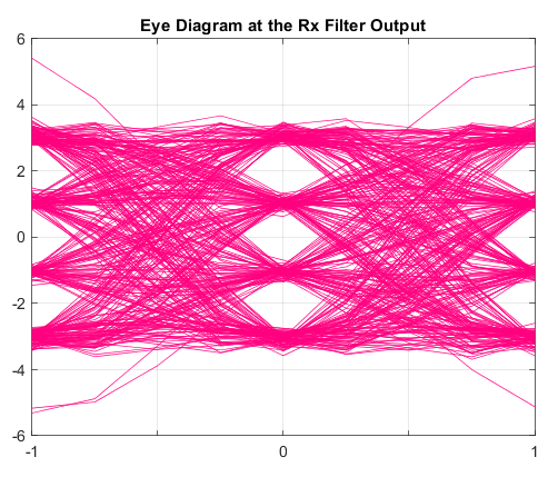
The final result is still an open eye diagram with clear symbols, albeit with moderate ISI even at a very high SNR. This is shown in the figure below.

From here onwards, like C4FM, a standard PAM receiver can demodulate the signal and detect the transmitted bits.
Conclusion
In conclusion, demodulating a CQPSK signal using a standard C4FM receiver is a viable, hardware-efficient method for achieving backward compatibility in P25 networks. This compatibility works because differential phase-deviation in CQPSK mimics the instantaneous frequency deviations of a four-level FSK (C4FM) signal over time. However, because CQPSK is a non-constant envelope modulation that possesses underlying amplitude variations, passing it through a C4FM frequency discriminator disregards these amplitude components.
On the one hand, this allows a basic FM-discriminator receiver to successfully decode the raw bitstream without a complex linear I/Q demodulator. On the other hand, it introduces a noticeable Bit Error Rate (BER) penalty and diminishes signal robustness in severe multipath or simulcast fading environments. Keep in mind that fully optimizing the spectral efficiency and range of a CQPSK broadcast requires a true linear and coherent quadrature receiver.