Effect of a Sampling Clock Offset on an OFDM Waveform

In an earlier article on the impact of a sampling clock offset on a single-carrier waveform, we explained the nature of a Sampling Clock Offset (SCO), i.e., a difference in sampling clock frequency between the Tx and the Rx. This is also known as a symbol timing frequency offset. The meaning of a sampling clock offset for a slow Rx clock that skips some samples within an interval is visually demonstrated in the figure below.

In the context of OFDM systems, a previous article describes how the normalized Carrier Frequency Offset (CFO) and the normalized Symbol Timing Offset (STO) affect the FFT input at the Rx. Now assuming a successful timing synchronization, we study the impact of the residual normalized CFO and a normalized Sampling Clock Offset (nSCO).

For a Rx sampling the waveform at sampling intervals of $\tilde T_S$ instead of $T_S$, a sampling clock offset and its normalized versions are defined as
$$\begin{equation*} \xi = \tilde T_S – T_S, \qquad \xi_0 = \frac{\tilde T_S – T_S}{T_S} = \frac{\xi}{T_S} \end{equation*}$$

The frequency of each OFDM subcarrier $k$ is given by $F_k=k\Delta_F$ where $\Delta_F$ is the subcarrier spacing. After the introduction of a residual CFO $F_\Delta$ and sampling at $t=n\tilde T_S$, we get
$$\begin{equation*} \begin{aligned} 2\pi(F_k +F_{\Delta})t\big|_{t=n\tilde T_S} \quad &= 2\pi\left(F_k + F_{\Delta}\right)n\tilde T_S \\ &= 2\pi\left(F_k + F_{\Delta}\right)\left(n\tilde T_S+nT_S-nT_S\right) \\ &= 2\pi\left(F_k + F_{\Delta}\right) \left(nT_S + n\frac{\tilde T_S-T_S}{T_S}T_S\right) \\ &= 2\pi\left(F_k + F_{\Delta}\right) \left(n + n\xi_0\right)T_S \\ &= 2\pi\frac{k\Delta_F + F_{\Delta}}{F_S} \left(1 + \xi_0\right)n \\ &= \frac{2\pi}{N}\left(k + \nu_0\right) \left(1 + \xi_0\right)n \end{aligned} \end{equation*}$$

where we have used a sampling rate of $F_S = N \Delta_F$. The quantity $\nu_0$ is defined as a normalized residual carrier frequency offset, i.e., the residual CFO $F_{\Delta}$ normalized by the subcarrier spacing $\Delta_F$.
$$\nu_0 = \frac{F_{\Delta}}{\Delta_F}$$

Next, this argument can be written as
$$\begin{align} 2\pi(F_k +F_{\Delta})t\big|_{t=n\tilde T_S} ~~ &= \frac{2\pi}{N}\left(k + \nu_0\right) \left(1 + \xi_0\right)n\nonumber \\ &= \frac{2\pi}{N} \left\{\underbrace{kn}_{\text{Term 1}} + \underbrace{\nu_0(1+\xi_0) n}_{\text{Term 2}} + \underbrace{(k\xi_0)n}_{\text{Term 3}} \right\}\label{eqOFDMntsd} \end{align}$$
Notice that the index $n$ is common to all the terms above, as opposed to the situation we encountered in timing offset synchronization before. As we saw in that case, these terms are handled as follows.

The DFT Argument

---

From the definition of the Discrete Fourier Transform (DFT),
$$X[k]=\sum_{n=0}^{N-1}x[n]e^{-j2\pi\frac{k}{N}n}$$

we observe that the FFT at the Rx consists of subcarriers with the arguments $-kn$ which simply cancels out Term 1 above.

Residual CFO Superimposed by the Drifting Clock

---

Being a function of time $n$, term 2 appears as a CFO equal to $\nu_0(1+\xi_0)$ at the FFT output. The part $\nu_0\cdot\xi_0$ is in addition to the original CFO $\nu_0$ and is very similar to the Doppler shift. Here, it is actually superimposed over the CFO by a moving or drifting Rx clock.

Impact of Sampling Clock Offset

---

This leaves Term 3 as a function of both $k$ and $n$. The data symbols at each subcarrier $k$ get rotated by the product of this index $k$ varying from $-N/2$ to $N/2-1$ with the SCO $\xi_0$ and this causes the constellation to rotate (recall that the constellation is in frequency domain in OFDM systems).

Consider the relation between the FFT size $N$, cyclic prefix length $N$ and the length of an OFDM symbol $N_{\text{OFDM}}$.
$$N_{\text{OFDM}} = N+N_{CP}$$

Here, sample number $n$ is equal to $mN_{\text{OFDM}}+N_{CP}$ at the start of $m^{th}$ OFDM symbol. Let us plug $n=mN_{\text{OFDM}}+N_{CP}$ in Eq ($\ref{eqOFDMntsd}$) above. After removal of Term 1 through an FFT at the Rx, we get
$$\begin{equation*} \begin{aligned} \text{Phase rotation} &= \frac{2\pi}{N}\Big\{\nu_0(1+\xi_0)+k\xi_0\Big\}n \\ &= \frac{2\pi}{N}\Big\{\nu_0(1+\xi_0)+k\xi_0\Big\}\left(mN_{\text{OFDM}} + N_{CP}\right) \end{aligned} \end{equation*}$$

In this discussion, we are ignoring extra noise arising from ICI and/or ISI for the sake of simplicity.

We can simplify our view of this effect if we only consider this phase rotation from the previous OFDM symbol to the present and denote it by $\varphi_\Delta[m]$. Assuming the same data symbols $a_{m-1}[k]$ $=$ $a_m[k]$ (which is the case for pilot subcarriers) and slowly varying channel $H_{m-1}[k]$ $\approx$ $H_m[k]$,
$$\begin{align*} \varphi_\Delta[m] &= \frac{2\pi}{N}\Big\{\nu_0(1+\xi_0)+k\xi_0\Big\}\Big\{mN_{\text{OFDM}} + N_{CP}\Big\} ~- \\ & \hspace{1in} \frac{2\pi}{N}\Big\{\nu_0(1+\xi_0)+k\xi_0\Big\}\Big\{(m-1)N_{\text{OFDM}} + N_{CP}\Big\} \\ &= \frac{2\pi}{N}\Big\{\nu_0(1+\xi_0)+k\xi_0\Big\}N_{\text{OFDM}} \\ &= 2\pi\Big\{\nu_0(1+\xi_0)+k\xi_0\Big\}\frac{N + N_{CP}}{N} \end{align*}$$

Let us denote
$$\begin{equation*} \lambda = \frac{N+N_{CP}}{N} \end{equation*}$$

so that the above equation becomes
$$\begin{equation}\label{eqOFDMphaseRotation} \varphi_\Delta[m] = 2\pi \lambda \Big\{\nu_0(1+\xi_0)+k\xi_0\Big\} \end{equation}$$

In other words, $\varphi_\Delta[m]$ $\propto$ $k\xi_0$. While this looks similar to the STO case where the phase rotation was equal to $k$ times the normalized symbol timing offset, the difference is that $k\xi_0$ is just the rotation between two consecutive OFDM symbols and keeps increasing with time.

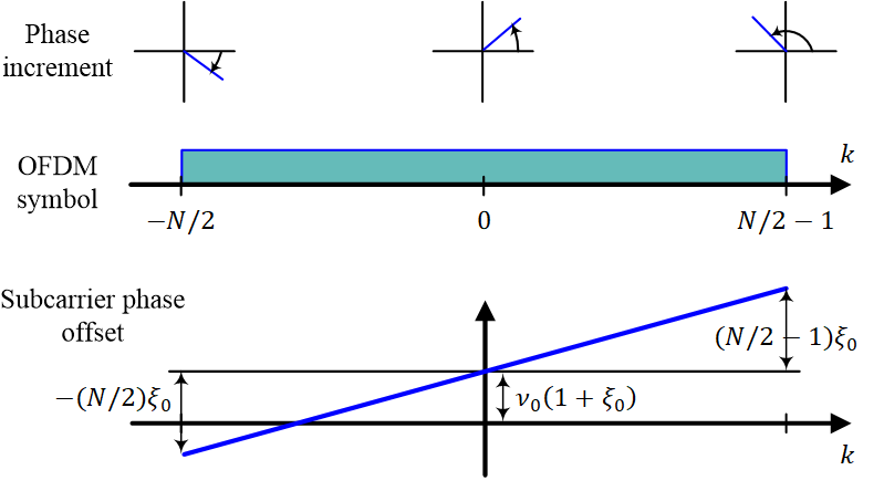
Ref. [1] draws the data symbols rotation at a subcarrier level corresponding to $\nu_0(1+\xi_0)+k\xi_0$ in an elegant manner which is the inspiration behind the figure below. Observe that the constant frequency shift is given by $\nu_0(1+\xi_0)$ while maximum rotation is experienced by the subcarriers at the edges of the spectrum, namely $k=-N/2$ and $k=N/2-1$, which are the leftmost and rightmost subcarriers, respectively.

In addition to the above, there is a sliding of the Rx FFT window due to the SCO between the Tx and Rx clocks. The details of such a window drift are similar to what was encountered in the context of single-carrier systems. A similar timing locked loop can stuff or delete an extra sample while slowly correcting for the SCO. For this purpose, an SCO error detector is needed. The documentation of QIRX software defined radio presents an excellent description of OFDM in general and a real world example of sampling clock misalignment in particular.

As a final remark, recall that we have included the effect of a residual carrier frequency offset here. One question is that why a perfect carrier frequency offset cannot be assumed in the system model (like the symbol timing offset). Recall from the timing synchronization problem in single-carrier systems that timing needs to be continuously adjusted and can almost never be set and done. Similar is the case with the frequency offset in an OFDM systems and a residual carrier frequency offset still needs to be included.

References

---

[1] M. Speth, S.A. Fechtel, G. Fock, H. Meyr, Optimum receiver design for wireless broad-band systems using OFDM – I, IEEE Transactions on Communications, Volume: 47, Issue: 11, November 1999.