 By
In signal processing applications, one frequently encounters the problem of estimating the frequency of a complex sinusoid embedded in noise. For example, a DSP engineer will encounter this problem in the delayed echo of an FMCW radar that directly translates into target range, or in carrier frequency estimation of a wireless communication system after timing synchronization has already been achieved (see Chapter 6 for details of how modulation removal exposes the underlying complex sinusoid).
Beyond communications and radar, this frequency estimation is also heavily relied upon in digital pitch tracking, speech synthesis, active and passive sonar detection, Doppler ultrasound and GNSS signal acquisition. Let us start with defining the problem.
A Sinusoid and the FFT
There are several methods to estimate the frequency of a simple sinusoid such as Kay, Fitz, LR and MM algorithms which rely on autocorrelation among the data samples. However, one of the most popular and straightforward methods is simply taking the Fourier Transform of the input sinusoid.
Since a Fourier Transform is defined in terms of complex sinusoids themselves, the spectrum of a complex sinusoid is a single impulse, and that of a real sinusoid is two impulses. But the Discrete Fourier Transform (DFT) in a machine can only work with a finite number of analysis frequencies $e^{j2\pi k/N}$ where $k$ goes from $0$ to $N-1$ (or $-N/2$ to $N/2-1$), as it is defined as
\[
X[k] = \sum_{n=0}^{N-1} x[n]e^{-j2\pi \frac{k}{N}n}, \qquad k = -N/2, \cdots, N/2-1
\]
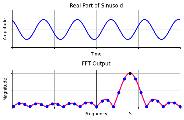
This leads us to the problem of peak search as follows. The DFT of any rectangular signal is a sinc signal. Since any finite duration signal can be thought of an infinite signal multiplied by a rectangular window, the result is the convolution of the signal spectrum with that of a sinc signal. In the case of a single sinusoid, when the signal frequency and one of the analysis frequencies are the same, there is an integer number of cycles within the signal duration and the exact peak of the sinc spectrum is sampled by the FFT. This is drawn in the figure below.
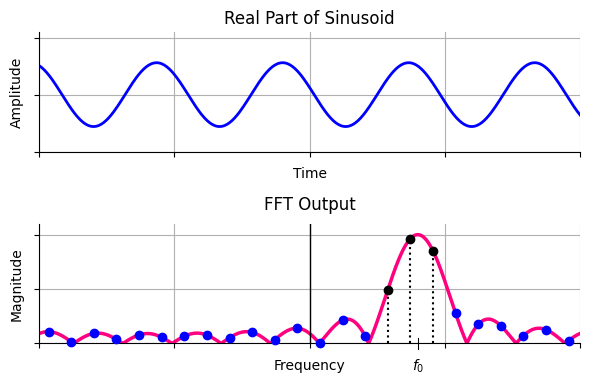
In real world, it is highly improbable that the particular frequency lies exactly in the bin center. This gives rise to DFT leakage, which causes the signal energy to leak into all other DFT output bins. This is drawn in the figure below. Note that the shape of the sinc function did not change as compared to the last figure above; the non-integer number of cycles of the input in time domain cause the sinc spectrum to be sampled at nonoptimal locations.
Next, we discuss how to get closer to this peak despite imperferct spectral sampling.
Large FFT Size
The simplest solution to finding this peak is to compute an FFT with a large value of $N$, known as the FFT size.
- The rationale in time domain is that as the number of analysis frequencies increases, one of them will have almost the same number of cycles within the signal span as the target frequency.
- In frequency domain, decreasing $1/N$ brings the spectral samples closer to each other, increasing the probability that one of them lies much closer to the actual peak.
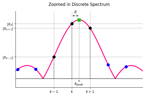
However, a large FFT size is an overkill for such an application. A simpler solution is to take a small FFT and then use a different algorithm that estimates the real peak with just a few computations. In practice, the input signal is first windowed with a suitable window and then magnitude squared of the DFT is computed before peak interpolation. This is drawn in the figure below.
Some of the most widely used peak interpolation algorithms in DSP applications are described next.
Peak Search Algorithms using Magnitudes
Let us denote the three consecutive integer indices around the peak in the above figure as $k-1$, $k$ (closest to the peak) and $k+1$ while the corresponding DFT values by $X_{k-1}$, $X_{k}$ and $X_{k+1}$. In all the methods described next, the fractional offset $\delta$ is computed first and then true estimated peak frequency is calculated as
k_{\text{peak}} = k +\delta
\]
where $k$ is the original index of the maximum bin corresponding to $|X_{k}|$.
We start with the simplest peak search algorithm that fits a parabola across the three DFT magnitudes in the neighborhood of the actual peak.
Parabolic Interpolation
This simple technique, also known as quadratic interpolation, works by assuming that the sinc spectrum is a parabola. Therefore, it fits a second-order polynomial through the largest discrete sample and its two immediate neighbors in the magnitude spectrum. Here, we derive the fractional bin offset as follows.
A standard parabola equation is defined as
\[
y(x) = ax^{2}+bx+c
\]
Note that the same results can be derived from a centered parabola equation as $y(x) = p(x-\delta)^2 + q$ where $\delta$ is the frequency difference between the peak and $|X_k|$. Assuming that the central sample is at $k=0$ and neighboring samples at $k=\pm 1$, the respective spectral magnitudes are $|X_{-1}|$, $|X_{0}|$ and $|X_{1}|$. We get the following system of equations.
\[
\begin{aligned}
|X_{-1}| &= a(-1)^2 + b(-1) + c\\
|X_{0}| &= a(0)^2 + b(0) + c\\
|X_{1}| &= a(1)^2 + b(1) + c
\end{aligned}
\]
These three equations with three unknowns can be put into matrix form as $\mathbf{y = Ax}$, from which we get
\[
\left[\begin{matrix}|X_{-1}|\\ |X_{0}|\\ |X_{1}|\end{matrix}\right] = \left[\begin{matrix}1&-1&1\\ 0&0&1\\ 1&1&1\end{matrix}\right]\left[\begin{matrix}a\\ b\\ c\end{matrix}\right]
\]
Since $\mathbf{x = A^{-1}y}$, the final result is given by
\[
\left[\begin{matrix}a\\ b\\ c\end{matrix}\right]=\left[\begin{matrix}\frac{|X_{1}|-2|X_{0}|+|X_{-1}|}{2}\\ \frac{|X_{1}|-|X_{-1}|}{2}\\ |X_{0}|\end{matrix}\right]
\]
Now to find the actual frequency estimate, we utilize the fact that the peak of the parabola occurs where its first derivative with respect to $x$ is equal to zero.
\[
\frac{d}{dx}\big[ax^2 + bx + c \big] = 2ax + b = 0
\]
Solving for $x$ gives the fractional offset $\delta= -b/2a$. Finally, substituting the values of $a$ and $b$ from above yields the fractional interval.
\[
\delta = \frac{1}{2}\cdot \frac{|X_{-1}| – |X_{1}|}{|X_{-1}| -2|X_{0}| + |X_{1}|}
\]
For the general case of peak at $k$, the final expression is given by
\delta = \frac{1}{2}\cdot \frac{|X_{k-1}| – |X_{k+1}|}{|X_{k-1}| -2|X_{k}| + |X_{k+1}|}
\end{equation}
Next, let us explore how the same idea can be extended to Gaussian interpolation.
Gaussian Interpolation
Here, the continuous peak profile is modeled using a standard Gaussian function.
\[
y(x) = A\cdot \exp \left(-\frac{(x-\delta)^{2}}{2\sigma ^{2}}\right)
\]
Taking the natural logarithm of both sides transforms the system as
\[
\ln [y(x)]=\ln (A)-\frac{(x-\delta)^{2}}{2\sigma ^{2}}
\]
From the above expression, we can conclude that a Gaussian curve in the linear domain transforms into a parabola in the logarithmic domain. As a consequence, standard quadratic interpolation on these natural log values yields a peak estimate similar to Eq (\ref{equation-parabolic-interpolation}).
\[
\delta = \frac{1}{2}\cdot \frac{\ln |X_{k-1}| -\ln |X_{k+1}|}{\ln |X_{k-1}|-2\ln |X_{k}|+\ln |X_{k+1}|}
\]
The next technique we discuss was invented by Rife and Boorstyn.
Rife-Boorstyn Method
Instead of using three bins, Rife-Boorstyn’s core formulation notices that the true peak lies explicitly between the maximum bin $X_k$ and its largest immediate neighbor, which is $X_{k+1}$ if $|X_{k+1}|>|X_{k-1}|$, and $X_{k-1}$ otherwise. For example, this neighbor is $X_{k+1}$ in the figure drawn before.
Since the shape is a spectral sinc (refer to the same figure above), the ratio of the magnitudes of the two maximum bins simplifies as
\[
\frac{|X_{k+1}|}{|X_{k}|}=\left[\frac{\sin (\pi (1-\delta))}{\pi (1-\delta)}\right] \bigg/ \left[\frac{\sin (\pi \delta)}{\pi \delta}\right]=\frac{\delta}{1-\delta}
\]
where we have used the identity $\sin(A – B) = \sin A\cos B – \cos A\sin B$. Solving this directly for $\delta$ provides the final equation.
\[
\delta =\frac{|X_{k+1}|}{|X_{0}|+|X_{k+1}|}
\]
Let us now pay our attention towards the techniques that employ complex valued spectral samples instead of their magnitudes.
Peak Search Algorithms using Complex Samples
We start with the method proposed by Eric Jacobsen.
Jacobsen Method
Jacobsen observed that the parabolic interpolator has a simple expression but it is statistically biased and performs poorly in the presence of noise. He suggested some simple changes by using the complex DFT values rather than the magnitudes that significantly improved it accuracy.
The expression for his peak frequency estimator is given as
\[
\delta \approx -\text{Re}\left(\frac{X_{k+1}-X_{k-1}}{2X_{k}-X_{k-1}-X_{k+1}}\right)
\]
Quinn Method
Quinn proposed an interpolation algorithm that works as follows.
Define $\alpha_1$ and $\alpha_2$ as
\[
\alpha_1 = \text{Re} \left\{\frac{X_{k-1}}{X_k}\right\} \qquad \text{and}\qquad \alpha_2 = \text{Re} \left\{\frac{X_{k+1}}{X_k}\right\}
\]
In a similar manner, define
\[
\delta_1 = \frac{\alpha_1}{1-\alpha_1} \qquad \text{and}\qquad \delta_2 = \frac{-\alpha_2}{1-\alpha_2}
\]
If both $\delta_1$ and $\delta_2$ are positive, then $\delta = \delta_2$, otherwise $\delta=\delta_1$.
This estimation method suffers from significant systematic interpolation error and an increased root-mean-square error when the true frequency of the sinusoid lies near the center of a DFT bin ($\delta \approx 0$).
His second method directly addresses this deficiency by introducing a highly optimized smoothing function $\kappa(x)$:
\[
\kappa(x) = \frac{1}{4} \ln \left( 3x^2 + 6x + 1 \right) – \frac{\sqrt{6}}{24} \ln \left( \frac{x + 1 – \sqrt{2/3}}{x + 1 + \sqrt{2/3}} \right)
\]
The final $\delta$ is obtained by averaging the base estimators and applying the correction to their squared values:
\[
\delta = \frac{\delta_1 + \delta_2}{2} + \kappa(\delta_1^2) – \kappa(\delta_2^2)
\]
MacLeod Method
MacLeod recognized that the magnitude spectrum of a single tone could be treated as a quadratic optimization problem if weighted properly by the real components of the cross-bin correlations.
First, calculate a cross-bin parameter $\gamma$ as
\[
\gamma =\text{Re}\left(X_{k+1}X_{k}^{*}-X_{k-1}X_{k}^{*}\right)
\]
Next, calculate the peak energy denominator component $\beta$ as
\[
\beta =\text{Re}\left(2|{}X_{0}|{}^{2}+X_{1}X_{0}^{*}+X_{-1}X_{0}^{*}\right)
\]
Dividing these two parameters isolates the variable used in the peak offset calculation.
\[
R=\frac{\gamma }{\beta }
\]
Then, the final estimate is given by
\[
\delta =\frac{\sqrt{1+8R^{2}}-1}{4R}
\]
Let us now turn our attention towards root mean square error simulations to compare their performance under different settings.
Performance Comparison
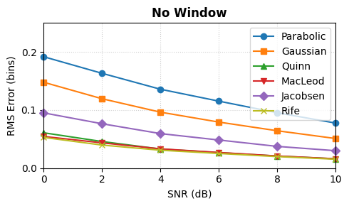
Considering the unwindowed (or rectangular window) case first for $\delta=0.5$, the figure below illustrates the Root Mean Square Error (RMSE) comparison of parabolic, Gaussian, Quinn, MacLeod, Jacobsen and Rife estimators. It is apparent that parabolic estimator has the worst performance while Quinn, MacLeod and Rife perform the best.
Digging deeper, however, reveals something more nuanced. Simulations across varying fractional frequency offsets ($\delta$) for a range of SNRs reveal that there is no single winner in all categories. For example, the figure below now plots the RMSE for $\delta=0$, $0.2$, $0.5$ and $0.7$ bins.
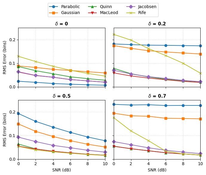
Regarding the plot, the following comments are in order.
- Impact of Fractional Offset $\delta$: When $\delta = 0$, all estimators experience a structural dip in RMSE due to perfect alignment with the FFT grid. As $\delta$ increases toward the worst-case scenario ($\delta = 0.5$), interpolation bias dominates the error budget for several estimators.
- Parabolic and Gaussian Estimators: These methods exhibit the highest structural bias when $\delta \neq 0$. Because they are fundamentally matched to specific quadratic profiles rather than the unwindowed sinc spectrum, they floor prematurely and underperform at high SNRs.
- Quinn and MacLeod Estimators: Both of these estimators display robust performance across all non-zero fractional offsets. They track closely together with MacLeod showing a marginal accuracy edge at lower SNR bounds due to its complex-domain formulation.
- Jacobsen Estimator: The Jacobsen method provides an excellent computational compromise. Its performance is close to the better estimators across all $\delta$ values shown here without requiring intensive non-linear function evaluations.
- Rife-Boorstyn Estimator: The Rife method is highly sensitive to the location of the tone. Interestingly, it achieves optimal precision at the worst-case boundary ($\delta = 0.5$) because its underlying model assumes the true peak lies exactly halfway between bins, but it exhibits severe thresholding degradation at off-center boundaries like $\delta = 0.2$ and $0.7$.
A summary of the above results is shown in the table below.
| Estimator | Performance, $\delta = 0$ | Performance, $\delta = 0.5$ | Computational Complexity | Robustness |
|---|---|---|---|---|
| Parabolic | Excellent | Poor (high bias) | Very low | Low |
| Gaussian | Excellent | Poor (high bias) | Moderate (logarithms) | Low |
| Quinn | Excellent | Optimal | Moderate | High |
| MacLeod | Excellent | Optimal | High (square roots) | Very high |
| Jacobsen | Excellent | Near-optimal | Low (linear only) | High |
| Rife-Boorstyn | Poor (thresholding) | Optimal | Low | Moderate |
Conclusion
In conclusion, different estimators can perform better under specific conditions but Jacobsen estimator proves to be a highly robust and low-complexity solution under all scenarios.
That being said, the input complex sinusoid is windowed in many scenarios before taking the FFT. Applying this window substantially changes the performance profile of these peak estimators. Why? Because it alters the underlying spectral shape from a sinc kernel to the Fourier Transform of the chosen window. To maintain optimal sub-bin precision in this scenario, specialized algorithms tailored to that specific window (e.g., the Modified Jacobsen or Windowed Quinn methods) must be substituted to eliminate model mismatch bias.