A wireless signal from one device to another travels through the use of electromagnetic waves propagated by an antenna. Electromagnetic waves have different frequencies and one can pick up a specific signal by tuning a radio Rx to a specific frequency. But what is a frequency anyway?
Watch the video below for an interesting description of actual time domain samples and how to interpret their frequency domain representation.
A Complex Sinusoid
Consider a complex number $V$ in an $IQ$-plane. A complex number is defined as a pair of real numbers in $(x,y)$-plane similar to the vectors but with different arithmetic rules (if you are interested in where these complex numbers come from, you can read my real-imaginative guide to complex numbers).
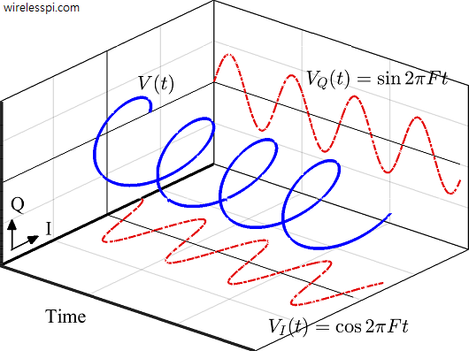
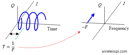
Now here imagine $V$ rotating anticlockwise in a circle at a constant rate with time as drawn in Figure below. We note the following.
- Instead of a complex number $V$, now $V(t)$ can be treated as a signal with time as independent variable and we call it a complex sinusoid.
- A constant rate implies that in any given duration $\Delta t$, the change in phase $\Delta \theta$ is a constant. This constant is known as the angular velocity and is defined as the rate of change in phase of this complex sinusoid, just like velocity is the rate of change of displacement.
\begin{equation*}
\text{angular velocity} = \frac{\Delta\theta}{\Delta t}
\end{equation*} - This angular velocity results in $V(t)$ rotating in the time $IQ$-plane and generating a helix, as shown in Figure above.
- The frequency of this complex sinusoid is defined as this angular velocity normalized by $2\pi$ so that the units are cycles/second instead of radians/second.
\begin{equation*}
F = \frac{1}{2\pi} \cdot \frac{\Delta \theta}{\Delta t}
\end{equation*}
Note that as time passes, $V(t)$ is shown in Figure above as coming out of the page. When its projection from a $3$-dimensional plane to a $2$-dimensional plane formed by time and $I$-axis is drawn downwards, we get its $I$ part $V_I(t)$ $=$ $\cos$ $2\pi F t$. Similarly, when the projection is drawn on a $2$-dimensional plane formed by time and $Q$-axis (on the back of the page), it generates the $Q$ part $V_Q(t)$ $=$ $\sin 2\pi F t$. Randomly choosing $\cos(\cdot)$ as our reference sinusoid, the $I$ component is called inphase because it is in phase with $\cos(\cdot)$ while $Q$ component is called qaudrature because $\sin(\cdot)$ is in quadrature — i.e.,$90^ \circ$ apart — with $\cos(\cdot)$.
In conclusion, a complex sinusoid with frequency $F$ is composed of two real sinusoids
\begin{aligned}
V_I(t)\: &= \cos 2\pi F t \\
V_Q(t) &= \sin 2\pi F t
\end{aligned}
\end{equation}\label{eqIntroductionComplexSinusoid}$$
where $F$ is the continuous frequency with units of cycles/second or Hertz (Hz). The direction of rotation is considered positive for anticlockwise rotation, and negative for clockwise rotation.
Amplitude $A$ and phase $\theta$ are the two other parameters that characterize a sinusoidal signal, where $A$ determines the maximum amplitude for the sinusoid, and $\theta$ determines the initial angular offset of $V(t)$ at $t=0$.
Remember that whenever you hear the word ‘frequency’, it is the frequency of a sinusoid $A\cos(2 \pi F t + \theta)$ or $A\sin(2 \pi F t + \theta)$. There are $3$ parameters that characterize a sinusoid:
- Frequency $\rightarrow$ $F$
- Phase $\rightarrow$ $\theta$
- Amplitude $\rightarrow$ $A$
It is clear that if the complex sinusoid $V(t)$ rotates with a frequency $F$, it completes $F$ cycles each second. In other words, it takes $1/F$ seconds to complete each cycle which is known as the time period $T$. Therefore, the frequency $F$ is related to time period $T$ as
\begin{align*}
F = \frac{1}{T}
\end{align*}
and the range of continuous frequency values is
\begin{equation}\label{eqIntroductionFreqRangeContinuous}
-\infty < F < \infty
\end{equation}
When one tunes to an FM radio station at $88$ MHz, one is actually listening to a station broadcasting a radio signal at a carrier frequency of $88\times10^6$ Hz, which means that the transmitter is oscillating at a frequency of $88,000,000$ cycles/second. Accordingly, that wave is completing one period in $T = 1/F = 11.4$ ns.
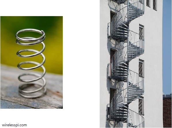
We find complex sinusoids everywhere such as in the form of a helical spring or round staircases!
What is a Negative Frequency?
Long ago, a lot of confusion clouded around negative numbers when numbers were used to count things. People could not understand how a person $A$ can give $-3$ apples to a person $B$. It turned out that this can be accomplished by changing the direction of giving, i.e., $A$ actually takes $3$ apples from $B$.
Similarly, a frequency is usually defined as an inverse period $F=1/T$ of a sinusoid. Naturally it becomes hard to visualize a negative frequency viewed as inverse period. Define it through the rate of rotation in anticlockwise direction of a complex sinusoid $V(t)$, and it is evident that a negative frequency simply implies rotation of $V(t)$ in a clockwise direction. For example, the complex sinusoid
\begin{equation*}
\begin{aligned}
\cos 2\pi (-F) t &= \cos 2\pi F t \\
\sin 2\pi (-F) t &= -\sin 2\pi F t
\end{aligned}
\end{equation*}
has a frequency of $-F$. Here, we have used the identities $\cos (-\theta) = \cos \theta$ and $\sin (-\theta) = -\sin \theta$.
Negative frequencies are a reality, just like negative numbers are a reality. Also note that from the definition of a complex conjugate, we can say that $V(t)$ is a complex sinusoid with frequency $F$ and $V^*(t)$ is a complex sinusoid with frequency $-F$.
A Real Sinusoid
We have learned that a complex sinusoid rotating in time $IQ$-plane generates two real sinusoids. The question is: How to produce only one real sinusoid in complex $IQ$-plane?
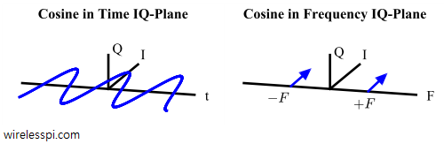
Interestingly, just like a complex sinusoid is made up of two real sinusoids as in Eq (\ref{eqIntroductionComplexSinusoid}), a real sinusoid can be produced by two complex sinusoids rotating in opposite directions to each other, $V(t)$ with a positive frequency $F$ and $V^*(t)$ with a negative frequency $-F$. Let us see how.
Figure below draws two complex sinusoids, $V(t)$ with a frequency $F$ shown as solid blue line while $V^*(t)$ with frequency $-F$ shown as dashed red line. Their $I$ and $Q$ components are similarly drawn as solid blue and dashed red lines, respectively. Observe that
- the $I$ parts exactly fall on top of each other and hence are the same $\cos 2\pi Ft$, whereas
- the $Q$ parts carry exactly the same amplitude with opposite signs to each other and hence are $\sin 2\pi Ft$ and $-\sin 2\pi Ft$, respectively.
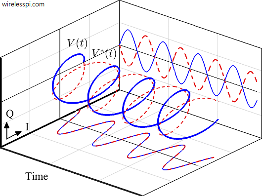
Consequently, when two such complex sinusoids are added together, the $I$ parts add up point-by-point while the $Q$ arms cancel out as a result of this addition.
This addition is a graphical representation of what we got from the following relation.
$$\begin{equation}
\begin{aligned}
\cos 2\pi Ft &= \frac{1}{2}\left\{V(t)+V^*(t) \right\} \\
0 &= \frac{1}{2}\left\{V(t)+V^*(t) \right\}
\end{aligned}
\end{equation}\label{eqIntroductionRealCosine}$$
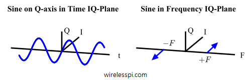
This figure is also a graphical representation of a sine wave that can be constructed in a similar manner by subtracting the two complex sinusoids.
$$\begin{equation}
\begin{aligned}
0 &= \frac{1}{2}\left\{V(t)-V^*(t) \right\} \\
\sin 2\pi Ft &= \frac{1}{2}\left\{V(t)-V^*(t) \right\}
\end{aligned}
\end{equation}\label{eqIntroductionRealSineQ}$$
This is somewhat similar to a double helix in a DNA molecule that carry the genetic instructions for our development. Maybe when the digital machines rise against us one day, they might be thinking of us as one of their own kinds.

Frequency Domain
We have talked about frequency being the rate of rotation of a complex sinusoid in time $IQ$-plane. It is evident that this rate of rotation can be changed from very slow (close to $0$) to as fast as possible (close to $+\infty$). Also, a clockwise direction of rotation implies a negative frequency, and hence the complete range of frequencies of a complex sinusoid is from $-\infty$ to $+\infty$. When a signal or function is drawn in frequency domain, the graph actually shows the $I$ and $Q$ components of those complex sinusoids whose frequencies are present in that signal. We begin with the simplest case of a complex sinusoid, then move towards a real sinusoid and then handle the most general case of an arbitrary signal.
[Complex sinusoid] Since one complex sinusoid has a single frequency, it is drawn as a single narrow impulse on the frequency $IQ$-plane in Figure below. The impulse is on $+F$ if the direction of rotation is anticlockwise and on $-F$ when the direction of rotation is clockwise. The impulse is at $-F$ in the figure due to the clockwise rotation in time domain.
[Real cosine] From what we learned above, a frequency domain representation of a cosine wave should be two impulses, one at frequency $+F$ due to $V(t)$ and the other at frequency $-F$ contributed by $V^*(t)$. This is illustrated in Figure below.
[Real sine] The case of a sine wave is slightly trickier. For the subtraction of two complex sinusoids, the result should be two impulses, one at frequency $+F$ due to $V(t)$ and the other at frequency $-F$ contributed by $V^*(t)$. However, the sign of $V^*(t)$ is negative and illustrated in Figure below. Consequently, notice that the sine wave exists on the time $Q$-axis.
A question is: what is the frequency domain representation of a sine wave on time $I$-axis? First, we say that a transform is utilized to go from time to frequency domain such as a Discrete Fourier Transform (DFT).
\begin{equation*}
\text{Time Domain}\quad \xrightarrow{\text{Transform}} \quad \text{Frequency Domain}
\end{equation*}
Next, we observe that rotating the time waveform of Figure above clockwise by $90^\circ$, the sine wave can be put on time $I$-axis. This will correspondingly rotate the frequency representation by $90^\circ$ clockwise (we can justify this step through the concept of linearity. It is just a phase rotation by $\exp\left(-j\pi/2\right)$ on both sides of the Transform (which is a multiplication by $-j$)). With this step, the frequency domain representation of a sine wave on time $I$-axis is plotted in Figure below.
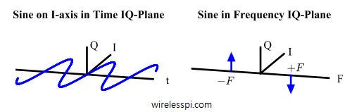
As a confirmation, we said that the inphase component implies a signal in phase with $\cos(\cdot)$. From the identity $\cos (A-90^\circ) = \sin (A)$, we can see why a sine wave is represented with a $-90^\circ$ phase rotation in frequency domain!
Visualizing the time and frequency $IQ$-planes is the single most important tool in understanding Digital Signal Processing (DSP) techniques. It will be of great help in devising algorithms for successful implementation of digital and wireless communications. If I assume that you can learn only one concept from this website and nothing else, I will recommend you departing with this skill.
In the above discussion, we saw that a complex sinusoid is represented by a single impulse in frequency domain. Two such complex sinusoids in time (and hence impulses in frequency) combine to form a real sinusoid. In frequency domain, we actually plotted the magnitudes through lengths and phases through orientations of those complex sinusoids. DSP folks can further explore the derivation for the spectrum of a sinusoid.
Similar is the case for signals composed of more than two complex sinusoids. As such, these complex sinusoids form a basic unit of signal construction of any shape and each `tick’ on the frequency axis represents the frequency of one participating complex sinusoid. As more and more of them come together, they form a continuum in frequency domain that is illustrated as a continuous spectral graph.
A natural question arises at this stage: What about the signals having components other than these nice looking sinusoids? The answer is surprising: There are hardly any! Long ago, scientists figured out that most signals of practical interest can be considered as a sum of many sinusoids — possibly infinite — oscillating at different frequencies regardless of the signal shape. So an arbitrary signal $s(t)$ can be written as
\begin{align*}
s(t) &= a_0 \sin (2\pi F_0 t) + a_1 \sin (2\pi F_1 t) + a_2 \sin (2\pi F_2 t) + \cdots \\
&= a_0 \sin (2\pi\frac{1}{T_0} t) + a_1 \sin (2\pi\frac{1}{T_1} t) + a_2 \sin (2\pi \frac{1}{T_2} t) + \cdots
\end{align*}
where $a_0$, $a_1$, $a_2$, $\cdots$, are amplitudes that determine the impact each sinusoid has on $s(t)$ while $1/T_0$, $1/T_1$, $1/T_2$, $\cdots$ are their respective frequencies. If $s(t)$ has no sinusoid of frequency $1/T_k$, then the corresponding amplitude $a_k = 0$.
It is difficult to believe in such a statement for many signals with sharp edges like a square or triangular waveform. Nonetheless, the concept is still true and the number of sinusoids participating in construction of such a signal tends to infinity. We now examine a few examples of such phenomena from everyday life.
- Wherever you are reading these lines, have a look around. You can spot only $3$ dimensions of space, namely $x$, $y$ and $z$ (the movie Interstellar captured the fourth dimension quite well and I am yet to see anything like that). Any point in space can be represented with a combination of just these $3$ basis components. Exactly in a similar but non-trivial way, almost all practical signals can be represented by a linear combination of the complex sinusoids and hence they are known as the basis signals.
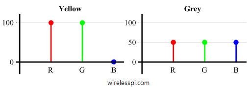
- Another good analogy is the RGB model in which Red, Green, and Blue colours combine together in various ways to reproduce a broad range of different colours. Figure below shows the `spectral’ contents of yellow and grey colours formed by contributions [100\% 100\% 0\%] and [50\% 50\% 50\%] from red, green and blue colours, respectively.
In the context of signals, consider a square wave which is a periodic signal. The curves in Figure below show how it is approximated with integer multiples of a fundamental frequency $F = 1/T$ (the corresponding negative axis in frequency domain is not shown for simplicity). The slowly varying curve riding on the square wave here consists of the first two terms
\begin{equation*}
s(t) = \sin(2 \pi F t) + \frac{1}{3}\sin( 2 \pi 3F t)
= \sin \left(2 \pi\frac{1}{T} t \right) + \frac{1}{3}\sin \left(2 \pi\frac{3}{T} t \right)
\end{equation*}
which is clearly quite inaccurate.
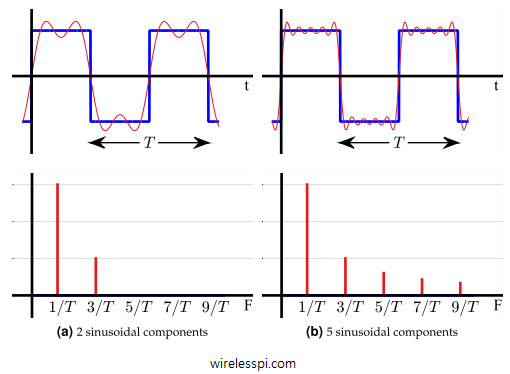
However, we can increase this approximation with just three more terms in the curve riding on the square wave as
\begin{align}
s(t) &= \sin(2 \pi F t) + \frac{1}{3}\sin(2 \pi 3F t) + \frac{1}{5}\sin(2 \pi 5F t) + \nonumber \\
& \hspace{2.2in} \frac{1}{7}\sin(2 \pi 7F t) + \frac{1}{9}\sin( 2 \pi 9F t) \nonumber \\
&= \sin \left(2 \pi\frac{1}{T} t \right) + \frac{1}{3}\sin \left(2 \pi\frac{3}{T} t \right) + \frac{1}{5}\sin \left(2 \pi\frac{5}{T} t \right) + \nonumber \\
& \hspace{2in} \frac{1}{7}\sin \left(2 \pi\frac{7}{T} t \right) + \frac{1}{9}\sin \left(2 \pi\frac{9}{T} t \right)\label{eqIntroductionSquareWave}
\end{align}
that displays significantly closer behaviour. If we increase the number of sinusoids with respective decreasing amplitudes, we can improve this approximation even further. Sometimes it is better to present this idea in a 3D figure to grasp the whole concept. Figure below draws the approximation of the square wave containing $5$ sinusoidal components on one side and the corresponding frequency domain representation on the other. Clearly, the meaning of all such waveforms adding together to generate the approximate square wave is more clear here.
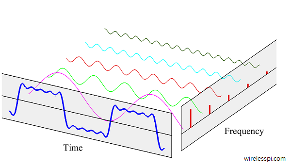
Now if you are confident that you have understood this concept, I want to shake it a little for a deeper appreciation. There is a slight misrepresentation in Figure above. The actual participants that add up are complex sinusoids, not the real sinusoids drawn in the figure. On the positive side of the spectrum, these complex sinusoids are rotating in an anticlockwise direction. On the negative side of the spectrum (not drawn), these are rotating in the clockwise direction. And the real sinusoids shown are just a special case due to this real and even square wave in time domain. All this would have been too complicated to draw in one such figure but you will gradually learn these concepts from the articles on this website.
This representation of periodic signals is known as Fourier series. For aperiodic signals, the period $T$ can considered as infinite, the spacing between these frequencies diminishes and a continuous frequency domain graph is obtained as the Fourier Transform. Here, we will not bother about Fourier series, Fourier Transform or Discrete-Time Fourier Transform. Instead, we will only focus on the Discrete Fourier Transform (DFT) that is actually computed in our digital machines.
Spectrum and Bandwidth
A frequency spectrum, or simply the spectrum, is just the range of all possible frequencies of electromagnetic radiation. A full continuous spectrum, for example, includes radio waves, microwaves, infrared, ultraviolet, x-rays and gamma rays. In the context of a signal, its spectrum contains the frequencies of complex sinusoids that sum up in time domain to form that signal.
In an ideal world, the bandwidth of a signal is the range of frequencies of complex sinusoids present in that signal. In other words, taking into account all the sinusoids, the bandwidth is simply the difference between the highest frequency $F_H$ and the lowest frequency $F_L$ in the spectrum of that signal.
\begin{equation}\label{eqIntroductionBW1}
\text{BW} = F_H – F_L
\end{equation}
An ideal band-limited signal has a spectrum that is zero outside a finite frequency range $F_L \le |F| \le F_H$:
\begin{equation}\label{eqIntroductionBW2}
S(F) = \left\{ \begin{array}{l}
0, \quad 0 \le |F| \le F_L \\
x, \quad |F_L| \le |F| \le |F_H| \\
0, \quad F_H \le |F| \le \infty \\
\end{array} \right.
\end{equation}
Having said that, a signal can have a very low contribution from a sinusoid of a particular frequency but not completely zero. Skipping the mathematical proof, we present the following argument: remember that the concept of frequency is defined through complex sinusoids that are infinitely long in time domain. Since sinusoids exist only for a finite duration in real-world, the spectrum of these truncated sinusoids is not an impulse anymore. Instead, frequency domain representation of a finite duration sinusoid spreads out in the entire spectrum from $-\infty$ to $+\infty$ and so does the ideal bandwidth of a time-limited signal.
A signal cannot be limited in both time and frequency domains. For practical implementations, a signal must be time limited which makes it unlimited in frequency. Therefore, every real signal occupies an infinite amount of bandwidth. A band-limited signal is then referred to as a signal with most of its energy concentrated within a certain amount of frequency range. Practical definitions of bandwidth vary depending on that amount of energy.
For example, Federal Communications Commission (FCC) defines bandwidth as the band in which $99 \%$ of the signal power is contained. Another common definition is that everywhere outside the specified band, a certain attenuation (say, $60$ dB) must be attained.
As a general rule, signals with fast irregular variations have large bandwidth as a large number of sinusoids are required to build such a signal, while slowly varying signals have low bandwidth. To test some of your own signals, you can see the code here.