This post is written on an advanced topic mainly for practitioners and researchers in the design of wireless systems. For learning about wireless communication systems from a DSP perspective (the idea behind SDRs), I recommend you have a look at my book.
F. M. Gardner described his well known Timing Error Detector (TED) — known as Gardner TED — in his often cited article [1]. Gardner was a pioneer in the area of synchronization and Phase Locked Loops (PLL). Later, M. Oerder (a student of Heinrich Meyr) derived this scheme from the maximum likelihood principle in [2]. Heinrich Meyr is the founder of the Institute for Integrated Signal Processing Systems at RWTH Aachen and one of the most respected scientists in communication engineering. His research results and methodology had a great impact on the design philosophy of single carrier systems in the last few decades.
In this article, I will mention an error in Oerder’s derivation that has the potential to cause confusion in understanding timing synchronization algorithms, which can be traced back to a longstanding misconception regarding the slope sign of the S-curve of a timing error detector. Let us explore it in detail.
Notations
Before we start this topic, I recommend that you read about Pulse Amplitude Modulation (PAM) for an introduction to pulse amplitude modulated systems, the framework in which timing synchronization algorithms are described here. The notations for the main parameters are the following.
- Sample time (inverse of sample rate): $T_S$
- Symbol time (inverse of symbol rate): $T_M$
- Data symbols: $a[m]$
- Square-root Raised Cosine pulse shape: $p(nT_S)$
- Raised Cosine pulse shape: $r_p(nT_S)$ (as it is the auto-correlation of a Square-Root Raised Cosine pulse)
- Timing error: $\epsilon _\Delta$
- Timing error estimate: $\hat \epsilon _\Delta$
System Model
Based on the notations above, such a pulse amplitude signal can be represented as
\[
s(t) = \sum _{i} a[i] p(t-iT_M)
\]
In the presence of a symbol timing offset $\epsilon _\Delta$, the received waveform is given by
\[
r(t) = \sum _{i} a[i] p(t-iT_M-\epsilon _\Delta)
\]
The receiver samples this waveform at times $nT_S+\hat \epsilon _\Delta$ where $\hat \epsilon _\Delta$ is its estimate of timing offset at that time. Therefore, the sampled received waveform in the absence of noise can be written as
\begin{equation*}
r(nT_S+\hat \epsilon _\Delta) = \sum _{i} a[i] p(nT_S+\hat \epsilon _\Delta-iT_M-\epsilon _\Delta)
\end{equation*}
In the above equation, we have ignored every other distortion at the Rx except for a symbol timing offset $\epsilon _\Delta$. This signal is input to a matched filter $h(nT_S) = p(-nT_S)$ and the output is written as
\begin{equation*}
z(nT_S+\hat \epsilon _\Delta) = \sum \limits _i a[i] r_p(nT_S+\hat \epsilon _\Delta -iT_M -\epsilon _\Delta)
\end{equation*}
Here, $r_p(nT_S)$ is the corresponding Nyquist pulse.
Maximum Likelihood Timing Error Detector (TED)
For unknown symbols, the likelihood function is maximum when the energy in the matched filter output $|z(nT_S+\hat \epsilon _\Delta)|^2$ is maximum. Taking its derivative at symbol $m$ and ignoring an irrelevant constant, the maximum likelihood Timing Error Detector (TED) is
\begin{equation}\label{eqSymbolCentricIdea}
e[m] = z(mT_M+\hat \epsilon _\Delta) \cdot \underbrace{z'(mT_M+\hat \epsilon _\Delta)}_{\text{drive this term towards zero}}
\end{equation}
It is evident that the maximum likelihood occurs where the derivative term approaches zero which coincides with the peak of the pulse for a single symbol and maximum eye opening for a shaped symbol stream.
Early-Late Timing Error Detector (TED)
For a Rx operating at $L=2$ samples/symbol, the second term in the maximum likelihood TED can be approximated with a differentiator computing only the first central difference, i.e., the term $z'(mT_M+\hat \epsilon _\Delta)$ can be approximated from one sample to the right (at $+T_M/2$) and one sample to the left (at $-T_M/2$) of the current time instant.
\[
z'(mT_M+\hat \epsilon _\Delta) \approx z\left(mT_M+\frac{T_M}{2}+\hat \epsilon _\Delta\right) –
z\left(mT_M-\frac{T_M}{2}+\hat \epsilon _\Delta\right)
\]
From Eq (\ref{eqSymbolCentricIdea}), this leads to an early-late approximation to the maximum likelihood TED known as Early-Late Timing Error Detector (EL-TED) as
\begin{align}\label{eqEL}
e[m] = z(mT_M+\hat \epsilon _\Delta) \left\{z\left(mT_M+\frac{T_M}{2}+\hat \epsilon _\Delta\right) –
z\left(mT_M-\frac{T_M}{2}+\hat \epsilon _\Delta\right)\right\}
\end{align}
The problem is that at the startup, the Rx does not know which sample out of $L=2$ samples corresponds to the symbol estimate $z(mT_M+\hat \epsilon _\Delta)$. Another sample like the one at $+T_M/2$ or $-T_M/2$ can easily be mistaken as the one corresponding to $T_M$.
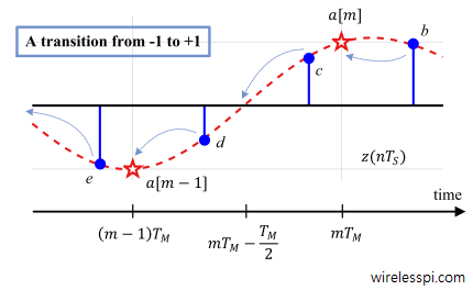
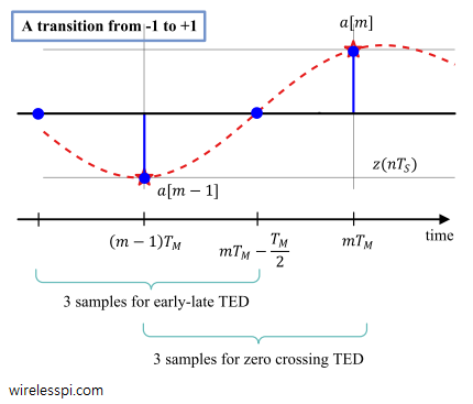
To answer this question, consider the figure below and apply the early-late equation for $b$, $c$ and $d$.
\begin{equation*}
e[m] = c\cdot (b-d) > 0
\end{equation*}

Consequently, it is treated as a case of early sampling $\hat \epsilon _\Delta<\epsilon _\Delta$. The timing loop would have shifted the sampling instant forward until $d$ is identified as the sample at $mT_M-T_M/2$. However, if the three TED samples were chosen as $c$, $d$ and $e$ at the start, \begin{equation}\label{eqELTEDexample} e[m] = d\cdot (c-e) < 0 \end{equation} and $d$ would have gone to instant $(m-1)T_M$ setting an underflow flag. We can say that in this game of $3$ samples, the middle sample always approaches the symbol center.
Zero Crossing Timing Error Detector (TED)
Now let us see what happens when a different TED is formed from the same samples as in Eq (\ref{eqELTEDexample}) but with a negative derivative term.
\begin{equation}\label{eqZCTEDexample}
e[m] = d\cdot\big\{-(c-e)\big\} = d\cdot (e-c) > 0
\end{equation}
Thus, the sampling instant will be pulled forwards until the middle sample $d$ reaches $mT_M-T_M/2$, i.e., in this game of $3$ samples, the middle sample approaches the zero crossing. Then, the left neighbouring sample $e$ will coincide with symbol $a[m-1]$ while the right neighbouring sample $c$ will coincide with $a[m]$. From this observation, Eq (\ref{eqEL}) and Eq (\ref{eqZCTEDexample}), we can write the expression for the new TED as
\begin{align}\label{eqGardner}
e[m] = z\left(mT_M-\frac{T_M}{2}+\hat \epsilon _\Delta\right) \cdot\Big\{z\left((m-1)T_M+\hat \epsilon _\Delta\right) – z\left(mT_M+\hat \epsilon _\Delta\right)\Big\}
\end{align}
which is nothing but the Gardner TED, a non-data-aided version of a general idea known as a Zero Crossing TED (ZC-TED).
The converging locations of the EL-TED and the ZC-TED are shown in the figure below. We conclude from Eq (\ref{eqZCTEDexample}) that negating the slope in a maximum likelihood TED makes the algorithm target the zero crossings of the waveform. While one of the samples aligns with the zero crossings, the other sample automatically aligns with the maximum eye opening due to $T_M/2$ spacing between them.
As opposed to the maximum likelihood perspective in Eq (\ref{eqSymbolCentricIdea}), the zero crossing idea works as follows.
\begin{equation}\label{eqZeroCrossingIdea}
e[m] = \underbrace{z(mT_M+\hat \epsilon _\Delta)}_{\text{drive this term towards zero}} \cdot \big\{-z'(mT_M+\hat \epsilon _\Delta)\big\}
\end{equation}
Clearly, Gardner TED is not an approximation of the maximum likelihood TED. It exploits the fact that the real purpose of a TED is not necessarily finding the maximum of the likelihood function but instead generating an error signal $e[m]$ that converges towards zero.
The Error and Clarification
However, [2] and numerous other references, including Gardner himself [1], have expressed the TED as
\begin{align}\label{eqGardner2}
e[m] = z\left(mT_M-\frac{T_M}{2}+\hat \epsilon _\Delta\right) \cdot
\Big\{z\left(mT_M+\hat \epsilon _\Delta\right) – z\left((m-1)T_M+\hat \epsilon _\Delta\right)\Big\},
\end{align}
a negative version of the one in Eq (\ref{eqGardner}). Applying a similar analysis as in Eq (\ref{eqELTEDexample}), such an expression eventually converges towards the EL-TED form in Eq (\ref{eqEL}).
Having these two different expressions, i.e., Eq (\ref{eqGardner}) and Eq (\ref{eqGardner2}), has been a source of confusion and has sometimes lead to erroneous application of the Gardner TED. Next, we discuss the root cause behind this difference in these expressions.
An S-curve for a carrier phase and carrier frequency error detector always has a positive slope at the origin. While many scientists also link the proper operation of a timing error detector with a positive slope at the origin, many others treat the S-curve as having a negative slope. The reason is as follows.
- A timing error $\epsilon _\Delta$ is introduced in a PAM waveform as
\begin{equation*}
z(t) = \sum \limits _i a[i] r_p(t -iT_M -\epsilon _\Delta)
\end{equation*}It is sampled at $t = nT_S+\hat \epsilon _\Delta$ which yields
\begin{align}
z(nT_S +\hat \epsilon _\Delta) &= \sum \limits _i a[i] r_p\Big[ nT_S+\hat \epsilon _\Delta -iT_M-\epsilon _\Delta\Big]\nonumber \\
&= \sum \limits _i a[i] r_p\Big[nT_S -iT_M-\epsilon _{\Delta:e}\Big]\label{eqTimingSyncNegTimingError}
\end{align}where
\begin{equation*}
\epsilon _{\Delta:e} \equiv \epsilon _\Delta-\hat \epsilon _\Delta
\end{equation*}When $\epsilon _{\Delta:e}>0$, i.e., $\epsilon _\Delta > \hat \epsilon _\Delta$, our estimate $\hat \epsilon _\Delta$ should increase. Similarly, when $\epsilon _{\Delta:e} < 0$, i.e., $\epsilon _\Delta<\hat \epsilon _\Delta$, our estimate $\hat \epsilon _\Delta$ should decrease: the resulting S-curve has a positive slope at the origin.
- On the other hand, some omit $\epsilon _\Delta$ from the incoming waveform as
\begin{equation*}
z(t) = \sum \limits _i a[i] r_p(t -iT_M)
\end{equation*}and assume that the Rx has the responsibility of properly adjusting the timing shift $\hat \epsilon _\Delta$. In this case, the matched filter output, again sampled at $t=nT_S+\hat \epsilon _\Delta$, is
\begin{equation*}
z(nT_S +\hat \epsilon _\Delta) = \sum \limits _i a[i] r_p\Big[nT_S-iT_M+ \hat \epsilon _\Delta\Big]
\end{equation*}The overall timing error, while having a negative sign in Eq (\ref{eqTimingSyncNegTimingError}), appears with a positive sign here. When our estimate $\hat \epsilon _\Delta<0$, it should increase. Similarly, when $\hat \epsilon _\Delta > 0$, it should decrease: the resulting S-curve has a negative slope at the origin.
The scientists following the former approach define Gardner TED as in Eq (\ref{eqGardner}) and EL-TED as in Eq (\ref{eqGardner2}) that converges to Eq (\ref{eqEL}). On the other hand, those following the latter approach define the Gardner TED as in Eq (\ref{eqGardner2}). The confusion between a Gardner TED and an EL-TED is thus clarified.
This lead [2] to mistaking the Gardner TED as another approximation to the maximum likelihood TED, although the real approximation was the EL-TED. Interestingly, this is what lead to Gardner himself deriving the TED in [1] through the former approach but then reversing the sign of the error signal at the last moment so that the TED slope could become negative at the origin. According to him, "the reversal of sign has no significance in the formal manipulations or in the processor’s computation burden, but assures negative slope at the tracking point of the detector output".
References
[1] F. M. Gardner, A BPSK/QPSK timing-error detector for sampled receivers, IEEE Transactions on Communications, Vol. 34, No. 5, May 1986.
[2] M. Oerder, “Derivation of Gardner’s timing-error detector from the maximum likelihood principle,”, IEEE Transactions on Communications, Vol. 35, No. 6, 1987.